樹狀資料結構 — 概念與模式
範圍 — 樹的概念、樹的種類,以及走訪順序的策略 — 講的是為什麼與選哪個,再加上那些不屬於單一模式模板的進階技巧(Morris 穿線、倍增法、換根)。模板本身放在 tree2.md。 另見 — 從這份文件拆出去的深入內容:tree_lca_distance.md — LCA、節點距離、父節點對照表與根到葉路徑模板;tree_codec.md — 子樹序列化與樹 ⟷ 字串的編解碼;tree_construction.md — 從走訪結果、字串與索引範圍建樹;tree_examples.md — 本頁教的模式所對應的 LC 實作檔案庫。 相鄰主題:tree2.md — 每個模式一份編號好、可直接複製的模板;binary_tree.md — 二元樹 DFS 的狀態流向與結構性模板;bst.md — 有序的樹;tree_backtrack.md — 回程時要還原狀態的根→葉路徑題。
LeetCode 題目清單
時間複雜度
| 資料結構 | 搜尋 | 插入 | 刪除 | 最小/最大 |
|---|---|---|---|---|
| 樹(一般) | O(n) | O(n) | O(n) | O(n) |
一般的樹(沒有順序保證)— 每個操作都可能走遍所有節點。平衡的樹會把這些降到 O(log n)。空間是儲存的 O(n) 加上遞迴堆疊的 O(h)。想看操作是 O(log n) 的有序樹,見 bst.md。
總覽
樹是一種階層式資料結構,由節點以邊相連而成,有一個根節點且沒有環。樹是電腦科學裡組織資料的基本工具。
關鍵性質
- 節點:存資料,並指向子節點
- 根:最上層、沒有父節點的節點
- 葉子:沒有子節點的節點
- 高度:從根到最深葉子的距離
- 深度:從根到某個特定節點的距離
- 複雜度:見上方的 Time Complexity 表格
樹的陣列表示法
樹可以用陣列有效率地表示,完全二元樹尤其適合:
# Tree Structure
      1
     / \
    2   3
   / \
  4   5

# Array Representation: [1, 2, 3, 4, 5]
# Index mapping:
# - Root at index 0
# - For node at index i:
#   - Left child at index 2*i + 1
#   - Right child at index 2*i + 2
#   - Parent at index (i-1)/2
參考資料
0) 核心概念
0-1) 樹的種類
基本樹型
| 種類 | 說明 | 關鍵性質 | 使用情境 |
|---|---|---|---|
| 一般樹 | 節點可以有任意多個子節點 | 結構彈性大 | 檔案系統、組織圖 |
| 二元樹 | 每個節點 ≤ 2 個子節點 | 結構單純、適合遞迴 | 運算式樹、決策樹 |
| 完全二元樹 | 除了最後一層外每層都填滿 | 用陣列表示很有效率 | 堆積、優先佇列 |
| 完美二元樹 | 每一層都完全填滿 | 共 2^h - 1 個節點 | 理論分析 |
| BST | 左 < 根 < 右 的順序 | 搜尋/插入/刪除 O(log n) | 搜尋操作、資料庫 |
| 堆積 | 父子之間有大小關係 | 取最小/最大很快 | 優先佇列、排序 |
| 字典樹 | 字串用的前綴樹 | 字串操作很有效率 | 自動補完、拼字檢查 |
0-2) 常見的樹模式 優先度 4/5 — 高價值 — 這裡有缺口就會掉關
九種一再出現的形狀。每一列都指出那個模式的程式碼放在唯一一個地方 — 在這一系列文件裡,沒有任何模式會被寫兩遍。
| # | 模式 | 核心想法 | 程式碼在 | 範例 |
|---|---|---|---|---|
| 1 | 路徑類 | 把累積值(總和、目前最大值、路徑)透過 DFS 參數往下帶 | tree_lca_distance.md — 根到葉路徑模板 | LC 112, 113, 257, 437, 1448 |
| 2 | 子樹驗證 | 後序 — 先驗證兩個子節點,父節點才做決定 | tree2 1.3) | LC 98, 101, 110 |
| 3 | 高度 vs 深度 | 高度由下往上算(後序);深度由上往下帶(前序) | 0-3) 由上而下 vs 由下而上 | LC 104, 111, 543 |
| 4 | 建樹 | 一種走訪給出結構,另一種給出位置;或是在選定的根把索引範圍切開 | tree_construction.md | LC 105, 106, 654, 108 |
| 5 | 序列化 | 編碼 = 回傳字串的 DFS;解碼 = 消耗前綴的遞迴下降 | tree_codec.md | LC 297, 449, 606, 536 |
| 6 | 往父節點走 | 建一張父節點對照表,把樹當成無向圖,再往四面八方 BFS | tree_lca_distance.md — 往父節點走的模式 | LC 863, 742, 1740 |
| 7 | 節點路徑 | 把每棵子樹指紋化成 val,left,right(null 用 #),再對字串做雜湊 |
tree_codec.md | LC 652, 572, 508 |
| 8 | 帶狀態的節點刪除 | 節點自己帶 isDeleted,父節點帶 isParentDeleted;父節點死掉而自己存活的節點,就變成森林的一個根 |
tree_examples.md — LC 1110 | LC 1110, 1325, 669 |
| 9 | 求節點距離 | 前序 DFS 把 depth 往下帶,命中時再往上回傳;-1 當作找不到的哨兵值,因為 0 是合法答案 |
tree_lca_distance.md — 節點之間的距離 | LC 1740, 863, 1123 |
模式 2 與 3 是所有樹遞迴的兩半,所以下面會完整展開;另外七個都只隔一頁,位置寫在表格裡。 參考(模式 2):Subtree Validation Video
0-3) 由上而下 vs 由下而上的 DFS — 解樹題的兩種策略 優先度 5/5 — 必備 — 幾乎每一輪面試都會出現
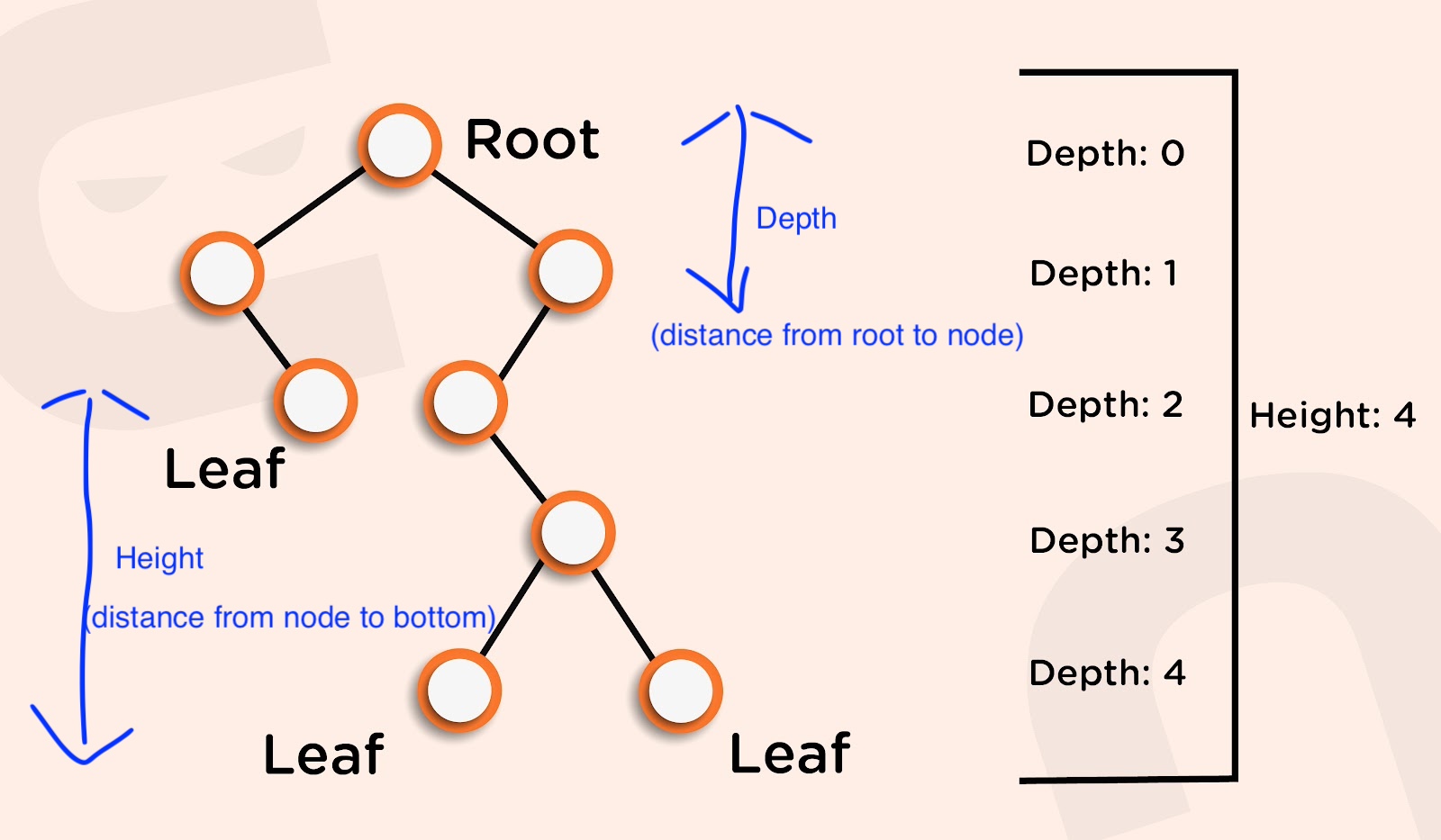
核心差別:
- 由上而下:用參數把狀態從父節點往下傳。答案在走訪過程中累積(前序位置)。
- 由下而上:用回傳值把結果從子節點往上收。答案在子樹解完之後才組出來(後序位置)。
Top-Down (Pre-order)                Bottom-Up (Post-order)
─────────────────────               ──────────────────────
      1  ← start here                    1  ← combine here
     / \  pass depth=1                  / \  return heights
    2   3  depth=2                     2   3  left=1, right=1
   / \     depth=3                    / \     left=2, right=0
  4   5  → update global max        4   5  → return max+1
模式 1:由上而下(把狀態往下傳,前序)
父節點把累積狀態(深度、路徑、目前最大值)交給子節點。通常會用全域變數或輸出參數來收最終答案。
// LC 104 — Top-Down: pass depth down, update global max
// 3 variants: (a) void helper + global var, (b) void helper + depth param, (c) return depth param

// Variant A: void helper + global var (simplest top-down)
int maxDepth = 0;

public int maxDepth_topDown(TreeNode root) {
    dfs(root, 1);       // start at depth 1
    return maxDepth;
}

private void dfs(TreeNode root, int depth) {
    if (root == null) return;

    // Pre-order position: update answer with current state
    maxDepth = Math.max(maxDepth, depth);

    // Pass depth+1 DOWN to children
    dfs(root.left, depth + 1);
    dfs(root.right, depth + 1);
}
模式 2:由下而上(把結果往上收,後序)
每個節點先問子節點要結果,再把它們組合起來。回傳值負責把答案往上帶。不需要全域變數。
// LC 104 — Bottom-Up: children return their depth, parent adds 1
public int maxDepth_bottomUp(TreeNode root) {
    if (root == null) return 0;

    // Post-order: solve children FIRST
    int leftDepth  = maxDepth_bottomUp(root.left);
    int rightDepth = maxDepth_bottomUp(root.right);

    // Combine: take max of children, add 1 for current node
    return 1 + Math.max(leftDepth, rightDepth);
}
比較:
| 面向 | 由上而下 | 由下而上 |
|---|---|---|
| 方向 | 根 → 葉(前序) | 葉 → 根(後序) |
| 狀態怎麼傳 | 靠參數(深度、路徑、最大值) | 靠回傳值 |
| 全域變數 | 常常需要 | 通常不用 |
| 輔助函式的回傳型別 | 常常是 void |
回傳算出來的值 |
| 心智模型 | 「我目前為止知道什麼?」 | 「我的子節點回報了什麼?」 |
| 程式碼簡潔度 | 比較囉嗦(多帶參數) | 比較精簡 |
什麼時候用哪一種:
Use TOP-DOWN when:
  → You need to pass parent/ancestor info to children
  → Path tracking: carry path, sum, or max-so-far downward
  → Early termination: can stop when condition met at a node
  → Examples: LC 112 (Path Sum), LC 129 (Sum Root to Leaf),
              LC 1448 (Count Good Nodes), LC 257 (Binary Tree Paths)

Use BOTTOM-UP when:
  → Answer depends on BOTH children's results
  → Need to compute subtree properties (height, size, balance)
  → Validation: check property holds for entire subtree
  → Examples: LC 104 (Max Depth), LC 110 (Balanced Tree),
              LC 543 (Diameter), LC 124 (Max Path Sum),
              LC 236 (LCA), LC 652 (Find Duplicate Subtrees),
              LC 968 (Binary Tree Cameras)
依策略分類的 LC 題目:
| LC # | 題目 | 由上而下 | 由下而上 | 備註 |
|---|---|---|---|---|
| 104 | Maximum Depth | Yes | Yes | 兩種都行;由下而上比較簡單 |
| 111 | Minimum Depth | Yes | Yes | 由下而上要防 null 子節點 |
| 110 | Balanced Binary Tree | - | Yes | 必須先檢查子樹高度 |
| 112 | Path Sum | Yes | - | 把剩餘的和往下帶 |
| 113 | Path Sum II | Yes | - | 由上而下 + 回溯 |
| 124 | Max Path Sum | - | Yes | 在每個節點把左右合起來 |
| 129 | Sum Root to Leaf Numbers | Yes | - | 把累積的數字往下帶 |
| 236 | Lowest Common Ancestor | - | Yes | 先在子樹裡找目標 |
| 257 | Binary Tree Paths | Yes | - | 把路徑字串往下帶 |
| 543 | Diameter of Binary Tree | - | Yes | 用全域變數追蹤 max(left+right) |
| 968 | Binary Tree Cameras | - | Yes | 貪婪三狀態:0=未覆蓋、1=有相機、2=已覆蓋 |
| 1448 | Count Good Nodes | Yes | - | 把目前最大值往下帶 |
混合模式:由下而上 + 全域變數
有些題目用由下而上的回傳值算子樹資訊,但同時維護一個全域變數來追蹤跨子樹的答案(例如直徑、最大路徑和)。
// LC 543 — Diameter: bottom-up height + global max update
int diameter = 0;

public int diameterOfBinaryTree(TreeNode root) {
    height(root);
    return diameter;
}

private int height(TreeNode root) {
    if (root == null) return 0;

    int left  = height(root.left);   // bottom-up: get children's height
    int right = height(root.right);

    // Global update: diameter passes THROUGH this node
    diameter = Math.max(diameter, left + right);

    // Return value: height of subtree (for parent to use)
    return 1 + Math.max(left, right);
}
面試提示:
LC 104(Max Depth)是同時練兩種策略最好的題目。先寫由下而上(三行),再改寫成由上而下(全域變數 + void 輔助函式)。兩種都懂,整套樹題工具箱就開了。
0-4) 走訪順序的選擇策略 優先度 5/5 — 必備 — 幾乎每一輪面試都會出現
When to use which traversal:

1. No specific root processing needed?
   → Any order works (preorder/inorder/postorder)

2. Need parent data for children?
   → Use PREORDER (root → left → right)

3. Need children data for parent?
   → Use POSTORDER (left → right → root)

4. Processing sorted data (BST)?
   → Use INORDER (left → root → right)

5. Level-by-level processing?
   → Use BFS/Level-order traversal

6. Need to move upward (to parent) or explore all directions?
   → Use MOVE PARENT pattern (Build parent map + BFS)

7. Need to compare or identify subtrees?
   → Use NODE PATH pattern (Subtree serialization with post-order)
收集葉子時該用前序還是後序(LC 872)
要收集葉節點時(例如 LC 872 Leaf-Similar Trees),任何先左後右的 DFS 順序都會得到同一串由左到右的葉子序列。不過實務上還是有差別:
前序(收集葉子時推薦):
private void getLeafSeq(TreeNode root, List<Integer> list) {
    if (root == null) return;

    // Check leaf BEFORE recursing into children
    if (root.left == null && root.right == null) {
        list.add(root.val);
        return;  // ← Early exit: skip 2 unnecessary null-child calls
    }

    getLeafSeq(root.left, list);
    getLeafSeq(root.right, list);
}
後序(也正確,但稍微浪費):
private void getLeafSeq(TreeNode root, List<Integer> list) {
    if (root == null) return;

    getLeafSeq(root.left, list);   // ← calls null, returns immediately
    getLeafSeq(root.right, list);  // ← calls null, returns immediately

    // Check leaf AFTER recursing (children were both null)
    if (root.left == null && root.right == null) {
        list.add(root.val);
    }
}
為什麼兩種結果一樣: 葉子序列只取決於「先左後右」的造訪順序,跟葉子檢查發生在什麼時候無關。葉子沒有子節點,所以後序對 null 的遞迴呼叫會在葉子檢查前立刻返回 — 葉子還是照同樣的由左到右順序被加進去。
為什麼比較推薦前序:
| 面向 | 前序 | 後序 |
|---|---|---|
| 葉子序列 | 左 → 右 | 左 → 右(一樣) |
| 在葉子提早返回 | 可以(加完就 return) |
不行(已經先遞迴進 null 子節點了) |
| 每個葉子多出的 null 呼叫 | 0 | 2 |
| 最適合 | 收集葉子、建路徑 | 求高度、子樹性質 |
面試時可以這樣答:
「我選前序,因為一旦判定是葉子就能立刻返回,省掉兩次對 null 子節點的多餘遞迴。任何先左後右的 DFS 都會得到同樣的葉子序列。」
其他「走訪順序會影響葉子/路徑收集」的相關題目:
| LC # | 題目 | 建議順序 | 為什麼 |
|---|---|---|---|
| 872 | Leaf-Similar Trees | 前序 | 在葉子提早返回 |
| 257 | Binary Tree Paths | 前序 | 由上而下建路徑 |
| 112 | Path Sum | 前序 | 把剩餘的和往下帶 |
| 104 | Maximum Depth | 後序 | 要先拿到子節點的高度 |
| 110 | Balanced Binary Tree | 後序 | 要驗證子樹高度 |
0-5) 走訪速查表(面試用) 優先度 4/5 — 高價值 — 這裡有缺口就會掉關
靈感來自 LC 113 Path Sum II — 關鍵洞見:選哪種走訪,就決定了演算法的結構。
| 走訪 | 順序 | 核心用途 | 什麼時候選它 |
|---|---|---|---|
| 前序 | 根 → 左 → 右 | 由上而下建路徑 | 根到葉的路徑、把父節點資訊帶給子節點、DFS + 回溯 |
| 後序 | 左 → 右 → 根 | 由下而上算子樹結果 | 高度/深度、子樹總和、最大路徑、樹上 DP |
| 中序 | 左 → 根 → 右 | 依排序順序處理節點 | BST 驗證、第 k 小、有序走訪 |
| BFS | 一層一層 | 逐層處理 | 最小深度、鋸齒走訪、右視圖、串接 next 指標 |
面試快速判斷
步驟 1 — 題目要什麼?
| 題目要的是… | 就用 |
|---|---|
| 所有根到葉的路徑/和為某值的路徑 | 前序 DFS + 回溯 |
| 計算和為目標的路徑數(起訖不限) | 前序 DFS + 前綴和雜湊表 |
| 樹高/最大深度 | 後序 DFS |
| 子樹性質(總和、大小、最大值) | 後序 DFS |
| 依結構辨識/比較子樹 | 後序 DFS + 序列化成 val,left,right + 雜湊表 |
| 找出重複的子樹 | 後序 DFS + 子樹序列化 + 雜湊表計數 |
| BST 的排序順序/第 k 小 | 中序 DFS |
| 驗證 BST | 中序 DFS |
| 逐層處理/最小深度 | BFS |
| 串接同一層的節點 | BFS |
面試小技巧(來自 LC 113):
題目要的是**「根 → 葉的路徑」,那幾乎一定是前序 DFS + 回溯**。
面試小技巧(來自 LC 437):
如果路徑不需要從根開始或在葉子結束,而且問的是數量, 就用前序 DFS + 前綴和雜湊表(樹上的「2-sum」模式)。 完整模板 — 為什麼回程時必須把 map 復原、基底情況的兩種寫法,以及 Java 中的
long溢位陷阱 — 見 prefix_sum_advanced.md 的 Template 14。
依走訪類型分類的經典 LC 題
前序 DFS + 回溯(根 → 葉的路徑)
| LC # | 題目 | 核心想法 |
|---|---|---|
| 112 | Path Sum | 前序 DFS,用剩餘的和在葉子做檢查 |
| 113 | Path Sum II | 前序 DFS + 回溯,收集所有路徑 |
| 257 | Binary Tree Paths | 前序 DFS + 回溯,組出字串路徑 |
| 437 | Path Sum III | 前序 DFS + 前綴和雜湊表,2-sum 技巧:查 map 裡有沒有 (curSum-target) — 模板 |
| 129 | Sum Root to Leaf Numbers | 前序 DFS,把累積的數字往下帶 |
| 404 | Sum of Left Leaves | 前序 DFS,把 isLeft 旗標往下帶;只有「以左子身分抵達的葉子」才加值 |
後序 DFS(由下而上算子樹)
| LC # | 題目 | 核心想法 |
|---|---|---|
| 104 | Maximum Depth of Binary Tree | 後序,回傳 max(left, right) + 1 |
| 543 | Diameter of Binary Tree | 後序,在每個節點追蹤最大的 left+right |
| 124 | Binary Tree Maximum Path Sum | 後序,追蹤穿過該節點的全域最大值 |
| 110 | Balanced Binary Tree | 後序,回傳高度,不平衡就回 -1 |
| 572 | Subtree of Another Tree | 後序序列化,或遞迴比對 |
| 236 | Lowest Common Ancestor | 後序,兩個目標都找到時回傳該節點 |
| 652 | Find Duplicate Subtrees | 後序 + 把子樹序列化成 val,left,right + 雜湊表 |
| 968 | Binary Tree Cameras | 後序貪婪,三種狀態:未覆蓋/有相機/已覆蓋 |
| 563 | Binary Tree Tilt | 後序,往上回傳子樹「總和」,同時把 abs(leftSum - rightSum) 累加到全域 — 經典的「回傳一個東西、蒐集另一個東西」 |
中序 DFS(BST/排序順序)
| LC # | 題目 | 核心想法 |
|---|---|---|
| 98 | Validate Binary Search Tree | 中序,檢查是否遞增 |
| 230 | Kth Smallest Element in BST | 中序走訪,數到第 k 個 |
| 501 | Find Mode in BST | 中序,追蹤 current/prev 與出現次數 |
| 538 | Convert BST to Greater Tree | 反向中序(右 → 根 → 左) |
| 700 | Search in a Binary Search Tree | 利用 BST 性質做中序搜尋 |
BFS/層序
| LC # | 題目 | 核心想法 |
|---|---|---|
| 102 | Binary Tree Level Order Traversal | 用佇列跑 BFS,逐層收集 |
| 111 | Minimum Depth of Binary Tree | BFS,第一次碰到葉子就回傳該層 |
| 116 | Populating Next Right Pointers | BFS 層序,把同層兄弟串起來 |
| 199 | Binary Tree Right Side View | BFS,取每層最後一個節點 |
| 103 | Zigzag Level Order Traversal | BFS + 每層交替方向 |
| 117 | Populating Next Right Pointers II | 在非完美樹上串接每層 — dummy-head 掃描,O(1) 空間(見模板 4-1) |
| 637 | Average of Levels in Binary Tree | BFS,每層加總後除以 levelSize |
| 987 | Vertical Order Traversal | 標上 (col, row, val),依 col → row → val 排序(見模板 4-2) |
1) 樹的模板與演算法
1.1) 通用樹模板 優先度 5/5 — 必備 — 幾乎每一輪面試都會出現
核心原則:樹題天生就是遞迴的 — 用子樹的解來解當前節點。
# Universal Tree Template
def solve_tree_problem(root, params):
    # Base case
    if not root:
        return base_case_value

    # Process current node (preorder position)
    process_current_node(root, params)

    # Recursively solve subtrees
    left_result = solve_tree_problem(root.left, updated_params)
    right_result = solve_tree_problem(root.right, updated_params)

    # Combine results (postorder position)
    result = combine_results(root, left_result, right_result)

    return result
// Java Universal Tree Template
public ResultType solveTreeProblem(TreeNode root, ParamType params) {
    // Base case
    if (root == null) {
        return defaultValue;
    }

    // Preorder: Process current node
    processCurrentNode(root, params);

    // Recursive calls
    ResultType leftResult = solveTreeProblem(root.left, updatedParams);
    ResultType rightResult = solveTreeProblem(root.right, updatedParams);

    // Postorder: Combine results
    ResultType result = combineResults(root.val, leftResult, rightResult);

    return result;
}
1.2) 模板選擇指南 優先度 4/5 — 高價值 — 這裡有缺口就會掉關
| 模式 | 模板 | 什麼時候用 | 範例題目 |
|---|---|---|---|
| DFS 遞迴 | 標準遞迴 | 大部分樹題 | LC 104, 110, 226 |
| DFS 迭代 | 用堆疊 | 避開遞迴深度限制 | LC 94, 144, 145 |
| BFS 層序 | 用佇列 | 需要逐層處理 | LC 102, 199, 515 |
| 分治法 | 由下而上遞迴 | 需要子樹的結果 | LC 124, 543, 687 |
| 路徑追蹤 | 帶路徑狀態的 DFS | 路徑相關題 | LC 112, 257, 437 |
| 往父節點走 | 父節點對照表 + BFS | 需要雙向探索 | LC 863, 742, 1740 |
| 節點路徑 | 子樹序列化 | 子樹比對/偵測 | LC 652, 572 |
1.3) 核心操作
1.3.1) 樹的走訪策略
兩大類作法:
-
深度優先搜尋(DFS) — 先往深處走,再往旁邊走
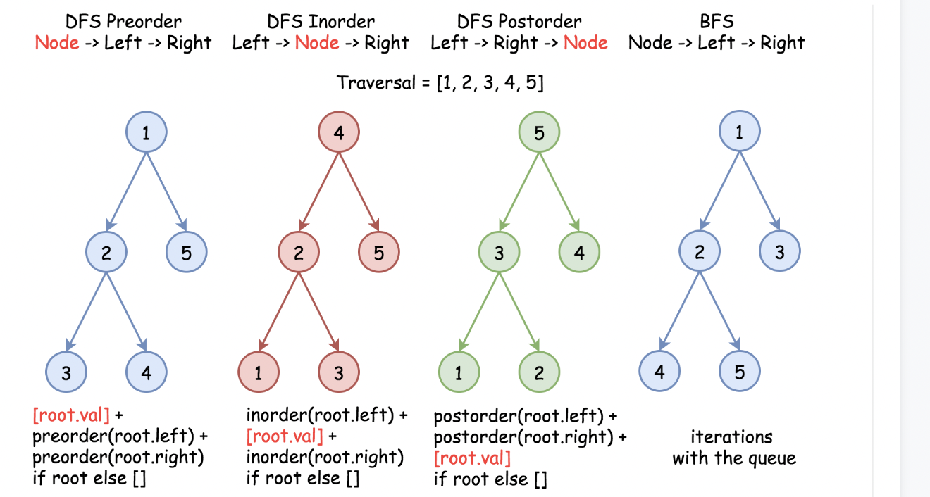
- 前序:根 → 左 → 右(由上而下處理)
- 中序:左 → 根 → 右(BST 上就是排序順序)
- 後序:左 → 右 → 根(由下而上處理)
-
廣度優先搜尋(BFS) — 一層一層處理
- 層序:先處理完深度 d 的所有節點,再處理 d+1
1.4) 走訪順序怎麼選
四種基本走訪的完整程式碼寫在 tree2.md — 那份文件是編號好的模板目錄,Python 與 Java 各一份,每個模式一份。 這裡要處理的是更前面的問題:到底該選哪一種。
| 答案取決於… | 走訪 | 為什麼 | 模板 |
|---|---|---|---|
| 父節點,而且在子節點的結果出來之前就要 | 前序 — 根 → 左 → 右 | 狀態往下流:一條路徑、一個深度、一個累積前綴 | tree2 1.1) — LC 144 |
| 這棵樹是 BST,而你要的是排序順序 | 中序 — 左 → 根 → 右 | BST 的中序就是排序後的序列,所以 LC 98 和 LC 230 各只要一行 | tree2 1.2) — LC 94 |
| 兩個子節點,節點才能給出答案 | 後序 — 左 → 右 → 根 | 狀態往上流:高度、總和、「這棵子樹合不合法」的判定 | tree2 1.3) — LC 145 |
| 到根的距離,或每一層各自的答案 | 層序(BFS) | 第一次碰到某節點走的一定是最短路徑,而一層就是佇列長度的一次快照 | tree2 1.4) — LC 102 |
| 一樣看層,但方向要交替 | BFS + 方向旗標 | 反轉那一列就好,不要去反轉走訪本身 | tree2 1.5) — LC 103 |
一句話的判斷法:問自己*「這個節點不用聽子節點回報,就能給出答案嗎?」* 可以 → 前序。不行 → 後序。「我需要一次拿到整排」→ BFS。
1.4-1) 不需要佇列的走訪
有兩種技巧能拿到一般走訪的答案,卻不用付出它的空間代價。它們不屬於單一模式的模板,所以留在這裡而不是放進目錄:
- O(1) 空間的逐層串接 — 節點本身已經有
next指標時,那一層自己就能當佇列用。完整寫在 tree2 8.1) — LC 116 / LC 117。 - 帶座標標註的走訪 — 在任何走訪中帶著
(row, col),最後再排序;走訪順序就變得不重要了, 這也是為什麼在垂直走訪、俯視/仰視圖與 LC 662 那種寬度索引題上,DFS 與 BFS 可以互換。 tree2 8.3) — LC 987。 - Morris 走訪 — 見下方。
模板 5:Morris 走訪(O(1) 空間的樹走訪)
用穿線二元樹做 O(1) 空間的中序走訪
核心概念: Morris 走訪把每個節點空著的右指標當成暫時的「線」,接回它的中序後繼節點,於是不用遞迴堆疊就能做到 O(n) 時間、O(1) 空間的走訪。
# In-order Morris Traversal — O(n) time, O(1) space
def inorderMorris(root):
    result = []
    curr = root
    while curr:
        if not curr.left:
            result.append(curr.val)
            curr = curr.right
        else:
            # Find in-order predecessor
            pred = curr.left
            while pred.right and pred.right is not curr:
                pred = pred.right
            if not pred.right:          # Thread: set predecessor → curr
                pred.right = curr
                curr = curr.left
            else:                        # Unthread: restore tree
                pred.right = None
                result.append(curr.val)
                curr = curr.right
    return result
# Pre/post-order variants follow the same thread-manipulation pattern.
// Java — Morris In-Order (LC 94)
// time = O(N), space = O(1)
public List<Integer> inorderTraversal(TreeNode root) {
    List<Integer> result = new ArrayList<>();
    TreeNode current = root;
    while (current != null) {
        if (current.left == null) {
            result.add(current.val);
            current = current.right;
        } else {
            TreeNode pred = current.left;
            while (pred.right != null && pred.right != current)
                pred = pred.right;
            if (pred.right == null) {   // first visit: create thread
                pred.right = current;
                current = current.left;
            } else {                    // second visit: unthread + process
                pred.right = null;
                result.add(current.val);
                current = current.right;
            }
        }
    }
    return result;
}
效能: O(n) 時間、O(1) 空間。面試官要求 O(1) 空間走訪時就用它。 前序變形: 在第一次造訪(建線的時候)就處理節點,而不是第二次。 後序: 需要反轉右脊 — 很複雜、幾乎不會考;還是用迭代堆疊比較實在。
| 走訪方法 | 時間 | 空間 | 會不會改動樹 |
|---|---|---|---|
| 遞迴 | O(n) | O(h) | 不會 |
| 迭代堆疊 | O(n) | O(h) | 不會 |
| Morris | O(n) | O(1) | 暫時會(之後還原) |
Morris 穿線家族 — 暫時的線 vs 永久的重接
上面的 Morris 走訪與 O(1) 空間的攤平(LC 114)共用同一個核心步驟:從當前節點出發,找到左子樹最右邊的節點(中序前驅),用它空著的 right 指標「穿線」到某處。兩者的差別只在拿這條線做什麼:
| 變形 | 線指向 | 會還原嗎? | 目的 | 例子 |
|---|---|---|---|---|
| Morris 走訪 | 中序後繼(curr) |
✅ 會(第二次造訪時拆線) | 用 O(1) 空間造訪節點 | LC 94, 144 |
| Morris 重接(攤平) | 原本的右子樹(curr.right) |
❌ 不會(永久) | 原地重整樹的結構 | LC 114 |
# Morris REWIRE pattern — permanent threading (LC 114 Flatten Binary Tree to Linked List)
# time = O(n), space = O(1)
def flatten(root):
    curr = root
    while curr:
        if curr.left:
            # find left subtree's rightmost node (in-order predecessor)
            rightmost = curr.left
            while rightmost.right:
                rightmost = rightmost.right
            # splice: predecessor.right -> original right subtree (PERMANENT, not restored)
            rightmost.right = curr.right
            curr.right = curr.left   # move left subtree to the right
            curr.left = None         # clear left
        curr = curr.right            # advance down the new right spine
心智模型: 對每個有左子節點的節點來說,左子樹被「插進」該節點與它原本的右子樹之間,因為左子樹的前序走訪必須緊接在該節點之後、右子樹之前。而左子樹最右邊的節點,正好就是右子樹該重新接回去的位置。
   curr                 curr
   /  \                    \
  L    R     ───►          L            (curr.right = curr.left)
   \                        \
    ...                     ...
      \                       \
     L_rightmost            L_rightmost
                              \
                               R         (L_rightmost.right = R)
遞迴版的對應寫法 — 後序遞迴,每次呼叫回傳它所攤平子樹的尾端,讓父節點知道要接在哪裡 — 詳見 tree_examples 16),包括為什麼尾端要依 右 → 左 → 節點 的順序檢查。
什麼時候該掏出這招: 任何「原地、O(1) 空間、沿著右脊重整樹」的題目。
while rightmost.right這個找前驅的步驟就是它的招牌。要認出它跟 Morris 走訪是同一套機械 — 只有線指向哪裡、以及要不要還原,這兩點不同。
1.5) 樹節點的初始化
# Python TreeNode Class
class TreeNode:
    def __init__(self, val=0, left=None, right=None):
        self.val = val
        self.left = left
        self.right = right

# Create a simple tree
root = TreeNode(1)
root.left = TreeNode(2)
root.right = TreeNode(3)
root.left.left = TreeNode(4)
root.left.right = TreeNode(5)
// Java TreeNode Class
public class TreeNode {
    int val;
    TreeNode left;
    TreeNode right;

    TreeNode() {}
    TreeNode(int val) { this.val = val; }
    TreeNode(int val, TreeNode left, TreeNode right) {
        this.val = val;
        this.left = left;
        this.right = right;
    }
}
2) 依模式分類的題目
2.1) 題型分類與模板 優先度 4/5 — 高價值 — 這裡有缺口就會掉關
走訪類題目
| 題目 | LC # | 模式 | 模板 | 難度 |
|---|---|---|---|---|
| Binary Tree Preorder Traversal | 144 | DFS 前序 | 前序模板 | Easy |
| Binary Tree Inorder Traversal | 94 | DFS 中序 | 中序模板 | Easy |
| Binary Tree Postorder Traversal | 145 | DFS 後序 | 後序模板 | Easy |
| Binary Tree Level Order Traversal | 102 | BFS 層序 | BFS 模板 | Medium |
| Binary Tree Zigzag Level Order | 103 | BFS 交替方向 | BFS + 方向 | Medium |
樹的性質類題目
| 題目 | LC # | 模式 | 模板 | 難度 |
|---|---|---|---|---|
| Maximum Depth of Binary Tree | 104 | DFS 由下而上 | 後序求高度 | Easy |
| Minimum Depth of Binary Tree | 111 | BFS/DFS | BFS 提早停止 | Easy |
| Balanced Binary Tree | 110 | DFS 檢查高度 | 高度驗證 | Easy |
| Symmetric Tree | 101 | DFS 比對 | 鏡像驗證 | Easy |
| Same Tree | 100 | DFS 比對 | 樹的比對 | Easy |
路徑類題目
| 題目 | LC # | 模式 | 模板 | 難度 |
|---|---|---|---|---|
| Binary Tree Maximum Path Sum | 124 | DFS 追蹤路徑 | 全域最大值更新 | Hard |
| Path Sum | 112 | DFS 路徑驗證 | 路徑累加 | Easy |
| Path Sum II | 113 | DFS 收集路徑 | 路徑 + 回溯 | Medium |
| Path Sum III | 437 | DFS 前綴和 | 路徑計數 | Medium |
| Sum Root to Leaf Numbers | 129 | DFS 路徑計算 | 路徑數值組合 | Medium |
| Count Good Nodes in Binary Tree | 1448 | DFS 路徑最大值 | 路徑狀態追蹤 | Medium |
| Diameter of Binary Tree | 543 | DFS 路徑長度 | 最長路徑 | Easy |
| Longest Univalue Path | 687 | DFS 路徑模式 | 同值路徑 | Medium |
距離與 LCA 類題目
| 題目 | LC # | 模式 | 模板 | 難度 |
|---|---|---|---|---|
| Lowest Common Ancestor | 236 | DFS 後序 | 標準 LCA | Medium |
| LCA of BST | 235 | BST 性質 | 數值比較 | Easy |
| Distance in Binary Tree | 1740 | LCA + 距離 | 路徑距離 | Medium |
| All Nodes Distance K | 863 | 圖 + BFS | 樹轉圖 | Medium |
| Smallest Subtree w/ Deepest Nodes | 865/1123 | LCA + 深度比較 | 回傳 (node, dist) 的 DFS | Medium |
高度與深度類題目
| 題目 | LC # | 模式 | 模板 | 難度 |
|---|---|---|---|---|
| Maximum Depth | 104 | DFS 由下而上 | 高度計算 | Easy |
| Minimum Depth | 111 | BFS/DFS | 到葉子的深度 | Easy |
| Balanced Binary Tree | 110 | DFS 高度驗證 | 平衡檢查 | Easy |
| Find Bottom Left Tree Value | 513 | BFS 層序 | 最深層最左節點 | Medium |
建樹類題目
| 題目 | LC # | 模式 | 模板 | 難度 |
|---|---|---|---|---|
| Construct Binary Tree from Preorder and Inorder | 105 | 分治 | 建樹 | Medium |
| Construct Binary Tree from Inorder and Postorder | 106 | 分治 | 建樹 | Medium |
| Serialize and Deserialize Binary Tree | 297 | 樹的編碼 | 字串轉換 | Hard |
| Construct String from Binary Tree | 606 | DFS 組字串 | 字串建構 | Easy |
改動樹結構的題目
| 題目 | LC # | 模式 | 模板 | 難度 |
|---|---|---|---|---|
| Invert Binary Tree | 226 | DFS 交換節點 | 翻轉樹 | Easy |
| Flatten Binary Tree to Linked List | 114 | DFS 重接結構 | 攤平樹 | Medium |
| Merge Two Binary Trees | 617 | DFS 合併 | 樹的合併 | Easy |
| Delete Nodes And Return Forest | 1110 | DFS + 狀態追蹤 | 刪節點並形成森林 | Medium |
子樹比對類題目(Node Path 模式)
| 題目 | LC # | 模式 | 模板 | 難度 |
|---|---|---|---|---|
| Find Duplicate Subtrees | 652 | Node Path 序列化 | 子樹雜湊 | Medium |
| Subtree of Another Tree | 572 | Node Path 比對 | 子樹配對 | Easy |
| Count Univalue Subtrees | 250 | Node Path 驗證 | 子樹性質檢查 | Medium |
2.2) 模式選擇指南
Problem Analysis Decision Tree:

1. Need to process all nodes?
   ├── Yes: Choose appropriate traversal (preorder/inorder/postorder/level-order)
   └── No: Continue

2. Need information from children for parent?
   ├── Yes: Use POSTORDER traversal
   └── No: Continue

3. Need information from parent for children?
   ├── Yes: Use PREORDER traversal
   └── No: Continue

4. Processing level by level?
   ├── Yes: Use BFS/Level-order traversal
   └── No: Continue

5. Need to move upward (to parent) or explore multi-directionally?
   ├── Yes: Use MOVE PARENT pattern (Build parent map + BFS)
   └── No: Continue

6. Need to compare or find duplicate subtrees?
   ├── Yes: Use NODE PATH pattern (Subtree serialization)
   └── No: Continue

7. Working with BST and need sorted order?
   ├── Yes: Use INORDER traversal
   └── No: Use any suitable approach
3) 總結與速查
3.1) 樹演算法複雜度總表
| 操作 | 平衡樹 | 非平衡樹 | 空間複雜度 |
|---|---|---|---|
| 搜尋 | O(log n) | O(n) | O(h) 遞迴 |
| 插入 | O(log n) | O(n) | O(h) 遞迴 |
| 刪除 | O(log n) | O(n) | O(h) 遞迴 |
| 走訪 | O(n) | O(n) | O(h) 遞迴 |
| 計算高度 | O(n) | O(n) | O(h) 遞迴 |
3.2) 走訪速查
| 走訪 | 順序 | 使用情境 | 關鍵特徵 |
|---|---|---|---|
| 前序 | 根 → 左 → 右 | 複製樹、序列化 | 先處理父節點再處理子節點 |
| 中序 | 左 → 根 → 右 | BST 的排序輸出 | 先左,再根,再右 |
| 後序 | 左 → 右 → 根 | 刪除樹、各種計算 | 先處理子節點再處理父節點 |
| 層序 | 一層一層 | 印出樹、最短路徑 | 用佇列,逐層處理 |
3.3) 解題模板
路徑追蹤模板
def solve_path_problem(root, target):
    def dfs(node, current_path, current_sum):
        if not node:
            return

        # Add current node to path
        current_path.append(node.val)
        current_sum += node.val

        # Check if we found target
        if not node.left and not node.right:  # Leaf node
            if current_sum == target:
                result.append(current_path[:])  # Add copy of path

        # Recurse to children
        dfs(node.left, current_path, current_sum)
        dfs(node.right, current_path, current_sum)

        # Backtrack
        current_path.pop()

    result = []
    dfs(root, [], 0)
    return result
3.4) 常見模式與技巧
高度 vs 深度模式
# Height (bottom-up, postorder)
def height(node):
    if not node:
        return 0
    return 1 + max(height(node.left), height(node.right))

# Depth (top-down, preorder)
def calculate_depth(node, depth=0):
    if not node:
        return

    node.depth = depth  # Assign depth to node
    calculate_depth(node.left, depth + 1)
    calculate_depth(node.right, depth + 1)
全域變數模式
class Solution:
    def __init__(self):
        self.max_sum = float('-inf')  # Global result

    def max_path_sum(self, root):
        def dfs(node):
            if not node:
                return 0

            left_max = max(0, dfs(node.left))   # Ignore negative paths
            right_max = max(0, dfs(node.right))

            # Update global maximum
            self.max_sum = max(self.max_sum, node.val + left_max + right_max)

            # Return maximum path through this node
            return node.val + max(left_max, right_max)

        dfs(root)
        return self.max_sum
3.5) 常見錯誤與提示 優先度 4/5 — 高價值 — 這裡有缺口就會掉關
🚫 常見錯誤:
- 遞迴忘了寫終止條件
- 走訪過程中錯誤地改動樹的結構
- 沒有妥善處理 null 節點
- 對題目選錯走訪順序
- 遞迴太深導致 stack overflow(改用迭代寫法)
✅ 最佳實務:
- 一律先檢查 null 節點
- 用 helper 函式來多傳幾個參數
- 樹很深時考慮改寫成迭代解
- 驗證輸入並處理邊界情況
- 變數名要有意義(left_result、right_result)
- 用平衡與非平衡的樹分別測試
3.6) 面試提示
- 釐清題目:問清楚 null 輸入、樹的結構、輸出格式
- 先寫遞迴解:多數樹題都有很漂亮的遞迴解
- 想想迭代版本:當遞迴深度可能出問題時
- 拿例子走一遍:用小例子驗證邏輯
- 分析複雜度:一定要討論時間與空間複雜度
- 處理邊界情況:空樹、單一節點、極深的樹
3.7) 相關主題
- 二元搜尋樹:順序性質讓操作變得有效率
- 堆積:具有堆積性質的完全二元樹
- 字典樹:字串操作用的前綴樹
- 線段樹:處理區間查詢問題
- 圖演算法:樹是圖的一種特例
進階樹技巧 — 倍增法、換根、Morris 走訪
倍增法(Binary Lifting)— 每次查詢 O(log n) 求 LCA 優先度 3/5 — 值得會 — 多半是必備模式的變形
import math

def build_binary_lifting(root, n):
    """Preprocess tree for O(log n) LCA queries."""
    LOG = max(1, int(math.log2(n)) + 1)
    parent = [[-1] * n for _ in range(LOG)]
    depth = [0] * n

    # BFS to set parent[0] and depth
    from collections import deque
    queue = deque([root.val])
    visited = {root.val}
    # ... (wire up parent[0][v] = direct parent of v)

    # Fill sparse table: parent[k][v] = 2^k-th ancestor of v
    for k in range(1, LOG):
        for v in range(n):
            if parent[k-1][v] != -1:
                parent[k][v] = parent[k-1][parent[k-1][v]]
    return parent, depth

def lca(u, v, parent, depth, LOG):
    # Bring u and v to the same depth
    if depth[u] < depth[v]: u, v = v, u
    diff = depth[u] - depth[v]
    for k in range(LOG):
        if (diff >> k) & 1:
            u = parent[k][u]
    if u == v: return u
    # Move both up until they meet
    for k in range(LOG - 1, -1, -1):
        if parent[k][u] != parent[k][v]:
            u = parent[k][u]; v = parent[k][v]
    return parent[0][u]
時間:預處理 O(n log n),每次 LCA 查詢 O(log n)。 適用:查詢量很大的 LC 236(LCA)、任兩點之間的路徑和。
換根 DP — 求出以每個節點為根時的答案
# LC 310 Minimum Height Trees — find roots minimizing tree height
# Equivalent: find centroid(s) of tree
def findMinHeightTrees(n, edges):
    if n == 1: return [0]
    from collections import defaultdict, deque
    graph = defaultdict(set)
    for u, v in edges:
        graph[u].add(v); graph[v].add(u)

    leaves = deque(i for i in range(n) if len(graph[i]) == 1)
    remaining = n
    while remaining > 2:
        remaining -= len(leaves)
        new_leaves = deque()
        while leaves:
            leaf = leaves.popleft()
            neighbor = next(iter(graph[leaf]))
            graph[neighbor].remove(leaf)
            if len(graph[neighbor]) == 1:
                new_leaves.append(neighbor)
        leaves = new_leaves
    return list(leaves)
樹的序列化/反序列化 — LC 297
前序 + null 標記的編解碼(Python 與 Java)、括號格式(LC 606/536)與深度前綴格式(LC 1028),見 tree_codec.md。
Morris 走訪(O(1) 空間)— 精簡版參考
完整的中序 Morris 模板(Python + Java)見上面的 Template 5: Morris Traversal。核心想法:把每個節點空著的 right 指標穿線到它的中序後繼,第二次造訪時再解除穿線 — O(n) 時間、O(1) 空間。前序/後序的變體用的是同一套穿線手法。
面試提示 — 樹
| 訊號 | 模式 |
|---|---|
| 「直徑/最長路徑」 | 後序:回傳高度,同時追蹤最大直徑 |
| 「最近共同祖先」 | 遞迴:若 root 就是其中一個目標節點,回傳 root |
| 「LCA 但查詢很多次」 | 倍增法(稀疏表) |
| 「以每個節點為根時的答案」 | 換根 DP(兩次 DFS) |
| 「序列化/反序列化樹」 | 前序 DFS 加 null 標記 |
| 「驗證 BST」 | 中序序列必須嚴格遞增 |
| 「用排序好的陣列建平衡 BST」 | 取中點遞迴 |
| 「O(1) 空間走訪」 | Morris 穿線 |
| 「任兩點之間的路徑和」 | 後序:追蹤通過每個節點的最大路徑 |