圖論演算法
範圍 — 圖的表示法、走訪、連通性、環偵測,以及一般圖題的完整目錄。 另見 — 從本檔拆出去的深入主題:graph_advanced.md — Tarjan(SCC、橋、關節點)、尤拉迴路、最大流/最小割、二分圖匹配與 k-著色;graph_examples.md — 解題存檔(LC 133 / 200 / 207 / 323 / 329 / 399 / 695 / 742 / 802 / 815 / 886 / 947 / 1319)。 鄰近文件:bfs.md — 廣度優先走訪;dfs.md — 深度優先走訪;topology_sorting.md — DAG 排序;union_find.md — 無向圖連通性;shortest_path_comparison.md — 怎麼挑帶權最短路徑演算法;Dijkstra.md — 非負權重;Bellman-Ford.md — 負權重/限制跳數;Floyd-Warshall.md — 全點對。
LeetCode 題目清單
總覽
圖論演算法是用來處理圖這種資料結構的技巧,圖由頂點(節點)和邊(節點之間的連結)組成。
關鍵性質
- 複雜度:見總結區的複雜度速查表
- 核心想法:把實體之間的關係與連結模型化
- 什麼時候用:網路問題、相依關係、路徑、連通性
- 關鍵演算法:BFS、DFS、Dijkstra、併查集、拓撲排序
核心特徵
- 有向 vs 無向:邊是單向還是雙向
- 帶權 vs 不帶權:邊有沒有成本
- 有環 vs 無環:圖裡有沒有環
- 連通 vs 不連通:是不是所有節點都互相可達
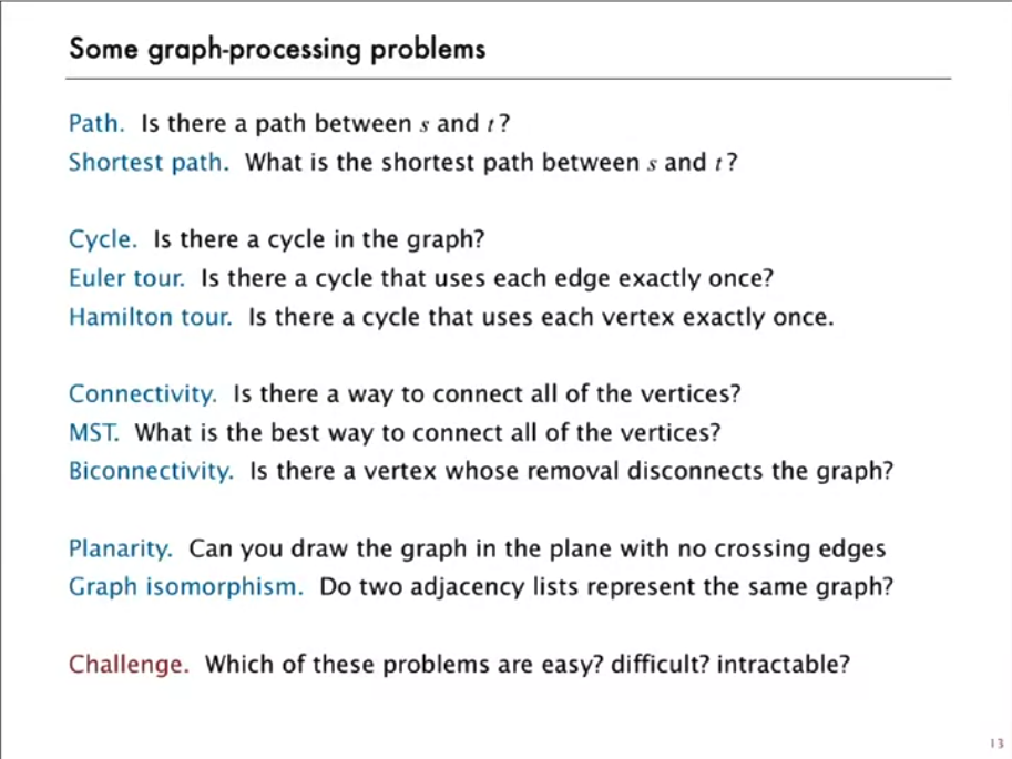
題型分類
類型 1:圖的走訪
- 說明:用 BFS 或 DFS 探訪所有節點
- 例題:LC 200(Number of Islands)、LC 133(Clone Graph)
- 模式:走遍每一個連通分量
類型 2:最短路徑
- 說明:求節點之間的最小距離
- 例題:LC 743(Network Delay)、LC 787(Cheapest Flights)
- 模式:Dijkstra、Bellman-Ford、Floyd-Warshall
類型 3:併查集(DSU)
- 說明:偵測環、找出連通分量
- 例題:LC 684(Redundant Connection)、LC 721(Accounts Merge)
- 模式:按秩合併、路徑壓縮
類型 4:拓撲排序
- 說明:替有相依關係的節點排序
- 例題:LC 207(Course Schedule)、LC 210(Course Schedule II)
- 模式:DFS 或 Kahn 演算法(BFS)
類型 5:二分圖
- 說明:檢查圖能不能只用兩種顏色著色
- 例題:LC 785(Is Graph Bipartite)、LC 886(Possible Bipartition)
- 模式:BFS/DFS 搭配著色
類型 6:最小生成樹
- 說明:用最小成本連通所有節點
- 例題:LC 1135(Connecting Cities)、LC 1584(Min Cost Connect Points)
- 模式:Kruskal 或 Prim 演算法
模板與演算法
哪個演算法歸哪份文件管 優先度 5/5 — 必備 — 幾乎每一輪面試都會出現
這份文件負責表示法、走訪、連通性與環偵測。每一個帶權或排序類的演算法都有專屬文件 — 要看實作就去那裡,別在這裡重推一次。
| 需求 | 這裡的模板 | 負責的文件 |
|---|---|---|
| 從 LC 的輸入格式建圖 | 下方的「圖的表示法」 | 本文件 |
| 走遍每個節點、數連通分量 | 模板 1 / 模板 2 | bfs.md、dfs.md |
| 最短路徑,不帶權 | 模板 1(BFS) | bfs.md |
| 最短路徑,帶權 | — | 見下方表格 |
| 替有相依關係的節點排序 | 模板 4(Kahn) | topology_sorting.md |
| 動態連通性、合併集合 | 模板 3(DSU) | union_find.md |
| 偵測環 | 模板 5 | 本文件 |
| 分成兩組/衝突著色 | 模板 6 | 本文件 |
| SCC、橋、關節點、尤拉迴路、最大流、k-著色 | — | graph_advanced.md |
| 每題一份完整解答 | — | graph_examples.md |
帶權最短路徑 — 看專屬文件
這些各自有完整的文件;在這裡再寫一次實作,正是害 graph.md 和它們脫節的原因。
| 需求 | 文件 | 複雜度 | 代表題 |
|---|---|---|---|
| 單源,非負權重 | Dijkstra.md | O((V+E) log V) | LC 743 |
| 單源,負權重/限制跳數/偵測負環 | Bellman-Ford.md | O(V·E) | LC 787 |
| 全點對,稠密圖 | Floyd-Warshall.md | O(V³) | LC 1334 |
| 不帶權,或 0-1 權重 | bfs.md — 一般 BFS/用雙端佇列的 0-1 BFS | O(V+E) | LC 1091, LC 1368 |
不確定要用哪個?→ shortest_path_comparison.md。
圖的表示法 — 怎麼建出來 優先度 5/5 — 必備 — 幾乎每一輪面試都會出現
幾乎每一道 LC 圖題丟給你的輸入,都逃不出那幾種形狀。認出形狀並把它轉成圖,就是解題的 頭三十秒。
| LC 輸入形狀 | 怎麼建 | 典型題目 |
|---|---|---|
edges = [[u,v], ...] |
鄰接串列,無向圖要建雙向 | LC 323, 684, 1971 |
edges = [[u,v,w], ...] |
存 (neighbor, weight) 配對的鄰接串列 |
LC 743, 787 |
isConnected[i][j] / graph[i][j] |
本來就是鄰接矩陣 | LC 547, 1334 |
graph[i] = [neighbors] |
本來就是鄰接串列 | LC 785, 797, 802 |
網格 char[][] / int[][] |
隱式圖 — 格子 = 節點,4 或 8 個鄰居 = 邊 | LC 200, 695, 1091 |
帶 neighbors 的 Node 物件 |
指標圖 — 用 {original: copy} 對照表走訪 |
LC 133 |
字串配對(["a","b"]) |
隱式圖 — 從輸入把節點挖出來丟進 defaultdict |
LC 399, 721 |
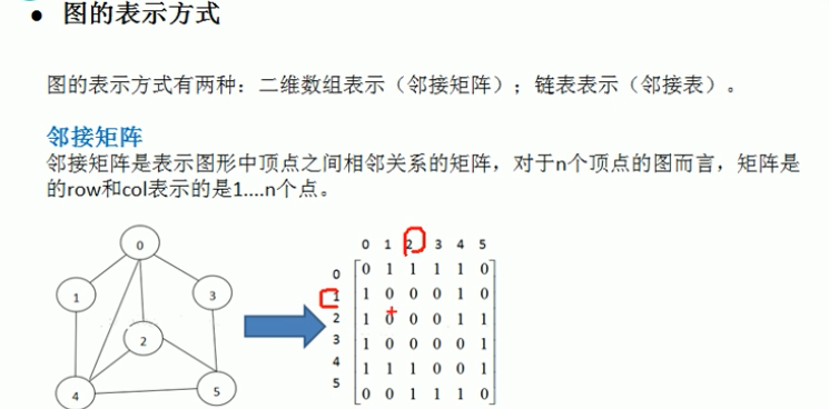
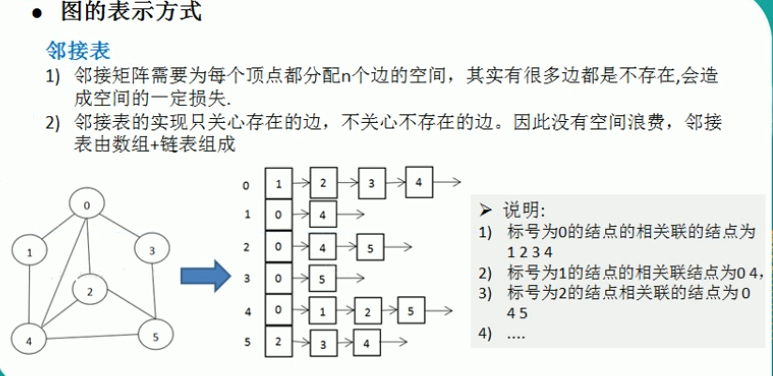
該選哪種表示法
| 空間 | 測試 u→v 這條邊 |
走訪 u 的鄰居 |
什麼時候用 | |
|---|---|---|---|---|
| 鄰接串列 | O(V + E) | O(deg u) | O(deg u) | 稀疏圖 — LC 的預設情況 |
| 鄰接矩陣 | O(V²) | O(1) | O(V) | 稠密圖,或 V 很小(Floyd-Warshall) |
| 邊串列 | O(E) | O(E) | O(E) | Kruskal、Bellman-Ford — 這類會掃過所有邊的演算法 |
邊串列完全不用建:題目丟給你的 edges 本身就是表示法。Kruskal 就排序它,
Bellman-Ford 就把它掃 V-1 次。
鄰接串列
# For edges list
graph = defaultdict(list)
for u, v in edges:
    graph[u].append(v)
    graph[v].append(u)  # Undirected

# For weighted edges
graph = defaultdict(list)
for u, v, w in edges:
    graph[u].append((v, w))
鄰接矩陣
# For unweighted
graph = [[0] * n for _ in range(n)]
for u, v in edges:
    graph[u][v] = 1
    graph[v][u] = 1  # Undirected

# For weighted
graph = [[float('inf')] * n for _ in range(n)]
for u, v, w in edges:
    graph[u][v] = w
把網格當成圖
# 4-directional movement
directions = [(0, 1), (1, 0), (0, -1), (-1, 0)]

# 8-directional movement
directions = [(0, 1), (1, 0), (0, -1), (-1, 0),
              (1, 1), (1, -1), (-1, 1), (-1, -1)]

# Check bounds
def is_valid(r, c, rows, cols):
    return 0 <= r < rows and 0 <= c < cols
有向 vs 無向,以及入分支度/出分支度
# undirected: add BOTH directions -- forgetting this is the most common graph bug
for u, v in edges:
    graph[u].append(v)
    graph[v].append(u)

# directed: one direction only, and degree splits into two counts
out_deg = [0] * n
in_deg = [0] * n
for u, v in edges:
    graph[u].append(v)
    out_deg[u] += 1
    in_deg[v] += 1
- 無向圖:
sum(degrees) == 2 * E。一棵樹剛好有V - 1條邊而且沒有環。 - 有向圖:源點的
in_deg == 0(Kahn 的起始集合,模板 4);匯點的out_deg == 0(LC 802 最終安全狀態)。 - 有些題目光靠分支度就能回答,根本不用走訪 — LC 997 Find the
Town Judge(
in == n-1 and out == 0)、LC 2924 Find Champion II(in == 0,而且唯一)、 LC 1361 Validate Binary Tree Nodes。這個模式與它的各種坑放在 topology_sorting.md。
通用圖模板
這是骨架,不是可執行的程式碼 — process_component 代表題目要你對每個連通分量做的事(數它、收集它、對它做彙總):
def graph_algorithm(n, edges):
    # Build adjacency list
    graph = collections.defaultdict(list)
    for u, v in edges:
        graph[u].append(v)
        graph[v].append(u)  # For undirected

    # Track visited nodes
    visited = set()

    # Process each component
    result = 0
    for node in range(n):
        if node not in visited:
            # Process component
            process_component(node, graph, visited)
            result += 1

    return result
visited 集合的紀律 優先度 4/5 — 高價值 — 這裡有缺口就會掉關
你在哪裡標記節點,決定了走訪會不會停下來、以及答案對不對。
- 入隊時標記,不是出隊時標記(BFS)。出隊才標記會讓同一個節點被塞進佇列很多次 — 結果還是對的,但最差情況會變成平方級。
- 要數節點或判斷可達性 → 一份共用的
visited集合;每個節點只處理一次。 - 要列舉所有路徑 → 不要共用集合;往下走時推入、往回走時彈出 (模板 2 的 LC 797 變形)。
- 有向圖的環偵測 → 三種狀態,不是布林值(模板 5)。
- 在網格上可以直接改輸入,不必另外配置
visited(grid[r][c] = '0')— 額外空間 O(1),但會毀掉輸入;面試時記得講出來。
三種記錄方式
# Set for simple visited
visited = set()

# Array for state tracking
# 0: unvisited, 1: visiting, 2: visited
state = [0] * n

# Dictionary for path reconstruction
parent = {}
模板 1:BFS 走訪 — LC 102
def bfs_template(graph, start):
    """Breadth-first search template"""
    from collections import deque

    visited = set([start])
    queue = deque([start])
    level = 0

    while queue:
        # Process level by level
        size = len(queue)
        for _ in range(size):
            node = queue.popleft()

            # Process node
            for neighbor in graph[node]:
                if neighbor not in visited:
                    visited.add(neighbor)
                    queue.append(neighbor)
        level += 1

    return level
模板 2:DFS 走訪 — LC 200 優先度 5/5 — 必備 — 幾乎每一輪面試都會出現
def dfs_template(graph, start):
    """Depth-first search template"""
    visited = set()
    path = []

    def dfs(node):
        visited.add(node)
        path.append(node)

        for neighbor in graph[node]:
            if neighbor not in visited:
                dfs(neighbor)

        # Backtrack if needed
        # path.pop()

    dfs(start)
    return visited
變形:列舉所有路徑(回溯,不用 visited 集合) — LC 797
變化點:這張圖是 DAG,所以根本沒有環要防 — 整個拿掉 visited 集合,改成推入/彈出目前的路徑(經典回溯)。在這裡用共用的 visited 集合是錯的:它會讓一個節點無法出現在多條路徑裡。
// java
// LC 797 - All Paths From Source to Target
// IDEA: DFS + backtracking on a DAG. No visited set (DAG => no cycles),
//       and a node may legitimately appear in many different paths.
// time = O(2^n * n), space = O(n) excluding output
import java.util.*;

public class Solution {
    public List<List<Integer>> allPathsSourceTarget(int[][] graph) {
        List<List<Integer>> res = new ArrayList<>();
        List<Integer> path = new ArrayList<>();
        path.add(0);                       // start node is always in the path
        dfs(graph, 0, path, res);
        return res;
    }

    private void dfs(int[][] graph, int u, List<Integer> path, List<List<Integer>> res) {
        if (u == graph.length - 1) {
            res.add(new ArrayList<>(path));   // NOTE: copy, not the live list
            return;
        }
        for (int v : graph[u]) {
            path.add(v);
            dfs(graph, v, path, res);
            path.remove(path.size() - 1);     // backtrack
        }
    }
}
# python
# LC 797 - All Paths From Source to Target
# IDEA: DFS + backtracking on a DAG (no visited set needed)
# time = O(2^n * n), space = O(n) excluding output
class Solution(object):
    def allPathsSourceTarget(self, graph):
        n = len(graph)
        res, path = [], [0]

        def dfs(u):
            if u == n - 1:
                res.append(path[:])    # copy!
                return
            for v in graph[u]:
                path.append(v)
                dfs(v)
                path.pop()             # backtrack

        dfs(0)
        return res

# [[1,2],[3],[3],[]] -> [[0,1,3],[0,2,3]]
經驗法則:數節點/判可達 → 用 visited 集合(每個節點一次)。列舉路徑 → 回溯,往下走時標記、往回走時取消標記。
模板 3:併查集(DSU) — LC 684 優先度 4/5 — 高價值 — 這裡有缺口就會掉關
class UnionFind:
    def __init__(self, n):
        self.parent = list(range(n))
        self.rank = [0] * n
        self.count = n

    def find(self, x):
        """Find with path compression"""
        if self.parent[x] != x:
            self.parent[x] = self.find(self.parent[x])
        return self.parent[x]

    def union(self, x, y):
        """Union by rank"""
        px, py = self.find(x), self.find(y)
        if px == py:
            return False

        if self.rank[px] < self.rank[py]:
            px, py = py, px
        self.parent[py] = px
        if self.rank[px] == self.rank[py]:
            self.rank[px] += 1

        self.count -= 1
        return True

    def connected(self, x, y):
        return self.find(x) == self.find(y)
模板 4:拓撲排序(Kahn 的 BFS) — LC 207 優先度 5/5 — 必備 — 幾乎每一輪面試都會出現
排序的各種變形 — 字典序、所有可能順序、平行排程、樹的重心、DAG 上的 DP — 都在 topology_sorting.md。
def topological_sort_bfs(n, edges):
    """Kahn's algorithm for topological sort"""
    from collections import deque

    graph = collections.defaultdict(list)
    indegree = [0] * n

    for u, v in edges:
        graph[u].append(v)
        indegree[v] += 1

    queue = deque([i for i in range(n) if indegree[i] == 0])
    result = []

    while queue:
        node = queue.popleft()
        result.append(node)

        for neighbor in graph[node]:
            indegree[neighbor] -= 1
            if indegree[neighbor] == 0:
                queue.append(neighbor)

    return result if len(result) == n else []
模板 5:環偵測 — 有向 vs 無向 優先度 4/5 — 高價值 — 這裡有缺口就會掉關
有向圖需要三種狀態,因為一個已經處理完的節點不代表有環 — 只有還留在目前 DFS 路徑上的節點才算。無向圖則完全不需要狀態:一條邊連到兩個已經在同一個連通分量裡的節點,那就是環。
兩段都是骨架 — n 和 graph 來自外層的解答,有向圖那段只列出遞迴的核心:
# Directed graph - DFS with states
def has_cycle_directed(graph):
    # 0: unvisited, 1: visiting, 2: visited
    state = [0] * n

    def dfs(node):
        if state[node] == 1:  # Back edge
            return True
        if state[node] == 2:
            return False

        state[node] = 1
        for neighbor in graph[node]:
            if dfs(neighbor):
                return True
        state[node] = 2
        return False

# Undirected graph - Union-Find
def has_cycle_undirected(edges):
    uf = UnionFind(n)
    for u, v in edges:
        if not uf.union(u, v):
            return True  # Already connected
    return False
連通分量其實是同一趟走訪,只是改成計數而不是搜尋 — 從每個還沒走訪過的節點各跑一次走訪,然後把計數器加一(上面的通用圖模板就是在做這件事)。LC 323、LC 547 和 LC 1319 的完整解法在 graph_examples.md。
模板 6:二分圖判定(2-著色) — LC 785 優先度 4/5 — 高價值 — 這裡有缺口就會掉關
定義:如果一張圖的頂點可以只用兩種顏色著色,而且沒有任何相鄰頂點同色,它就是二分圖。等價於檢查圖裡有沒有奇數長度的環。
時間複雜度:O(V + E) — 每個頂點和每條邊各走一次 空間複雜度:O(V) — 顏色陣列加上佇列/遞迴堆疊
使用情境:
- 圖著色問題
- 匹配問題(分派、排程)
- 衝突偵測
- 資源配置
- 網路流問題
關鍵性質:
- 所有的樹都是二分圖
- 有奇數環的圖不是二分圖
- 完全二分圖 K(m,n) 是二分圖
- 可以用 BFS 或 DFS 搭配 2-著色解決
解法 1:BFS 著色
def is_bipartite_bfs(graph):
    """Check if graph is bipartite using BFS"""
    from collections import deque

    n = len(graph)
    colors = [-1] * n  # -1: uncolored, 0: color A, 1: color B

    # Handle disconnected components
    for start in range(n):
        if colors[start] != -1:
            continue

        # BFS coloring
        queue = deque([start])
        colors[start] = 0

        while queue:
            node = queue.popleft()

            for neighbor in graph[node]:
                if colors[neighbor] == -1:
                    # Color with opposite color
                    colors[neighbor] = 1 - colors[node]
                    queue.append(neighbor)
                elif colors[neighbor] == colors[node]:
                    # Same color conflict - not bipartite
                    return False

    return True
解法 2:DFS 著色
def is_bipartite_dfs(graph):
    """Check if graph is bipartite using DFS"""
    n = len(graph)
    colors = [-1] * n

    def dfs(node, color):
        colors[node] = color

        for neighbor in graph[node]:
            if colors[neighbor] == -1:
                # Recursively color with opposite color
                if not dfs(neighbor, 1 - color):
                    return False
            elif colors[neighbor] == colors[node]:
                # Same color conflict
                return False

        return True

    # Check each component
    for i in range(n):
        if colors[i] == -1:
            if not dfs(i, 0):
                return False

    return True
用併查集偵測二分圖、最大二分圖匹配和貪婪 k-著色都在 graph_advanced.md;LC 886 Possible Bipartition 的完整解法在 graph_examples.md。
效能比較
| 解法 | 時間 | 空間 | 最適合的情境 |
|---|---|---|---|
| BFS | O(V+E) | O(V) | 一層一層處理 |
| DFS | O(V+E) | O(V) | 簡潔的遞迴寫法 |
| 併查集 | O(E⋅α(V)) | O(V) | 動態的衝突偵測 |
| 網格專用 | O(R⋅C) | O(R⋅C) | 二維網格問題 |
常見模式與技巧
模式辨識:
- 圖著色 → 二分圖判定
- 衝突/相容性 → 建一張衝突圖
- 分成兩組 → 二分圖分割
- 匹配問題 → 二分圖匹配
實作技巧:
- 一定要處理不連通的分量
- 顏色一律用 0/1 或 -1/1,保持一致
- 著色的當下就馬上檢查衝突
- 動態情境考慮改用併查集
邊界情況:
- 空圖(依定義是二分圖)
- 單一節點(是二分圖)
- 沒有邊(是二分圖)
- 自環(只要存在就不是二分圖)
- 不連通的分量(每個都要檢查)
總結與速查
決策表 — 該用哪個圖的模式?
Graph Algorithm Selection Flowchart:

1. What is the problem asking for?
   ├── Find shortest path → Continue to 2
   ├── Check connectivity → Use Union-Find or DFS/BFS
   ├── Order with dependencies → Use Topological Sort
   ├── Detect cycles → Use DFS with states or Union-Find
   └── Traverse all nodes → Use BFS or DFS

2. For shortest path problems:
   ├── Unweighted graph → Use BFS
   ├── Non-negative weights → Use Dijkstra
   ├── Negative weights → Use Bellman-Ford
   └── All pairs → Use Floyd-Warshall

3. For connectivity problems:
   ├── Static graph → Use DFS/BFS once
   ├── Dynamic connections → Use Union-Find
   └── Count components → Use either approach

4. For traversal problems:
   ├── Level-by-level → Use BFS
   ├── Path finding → Use DFS with backtracking
   └── State space search → Use BFS for optimal

5. Is the graph special?
   ├── Tree → Simpler DFS/BFS
   ├── DAG → Topological sort possible
   ├── Bipartite → Two-coloring
   └── Grid → Treat as implicit graph
複雜度速查
| 演算法 | 時間複雜度 | 空間複雜度 | 備註 |
|---|---|---|---|
| BFS/DFS | O(V + E) | O(V) | 標準走訪 |
| Dijkstra | O((V+E)logV) | O(V) | 搭配二元堆積 |
| Bellman-Ford | O(VE) | O(V) | 可處理負權重 |
| Floyd-Warshall | O(V³) | O(V²) | 全點對 |
| 併查集 | O(α(n)) | O(V) | 近似常數 |
| 拓撲排序 | O(V + E) | O(V) | 線性時間 |
面試訊號 → 模式
| 訊號 | 模式 |
|---|---|
| 「最短路徑,非負權重」 | Dijkstra |
| 「最短路徑,負權重/有環」 | Bellman-Ford |
| 「全點對最短路徑」 | Floyd-Warshall |
| 「課程先修條件、排順序」 | 拓撲排序(Kahn 的 BFS) |
| 「連通分量、合併」 | 併查集 |
| 「移掉某條邊/某個點會讓圖不連通」 | 橋/關節點(Tarjan) |
| 「最大流、二分圖匹配」 | Ford-Fulkerson / Edmonds-Karp |
| 「數島嶼、洪水填充」 | 網格上的 DFS/BFS |
| 「每條邊/每次轉移都恰好用一次」 | 尤拉迴路 — Hierholzer(LC 753, 332) |
| 「比值/換算/匯率查詢」 | 帶權 DFS 或帶權併查集(LC 399) |
| 「最長路徑,但每步都必須嚴格遞增」 | 隱式 DAG → DFS + 記憶化(LC 329) |
| 「因為共用同一列/同一個 email/同一個屬性而相連」 | 把該屬性也當成 DSU 的節點(LC 947, 721) |
| 「列舉每一條路徑,不只是判斷可達」 | DFS + 回溯,不用共用的 visited 集合(LC 797) |
依模式分類的題目
圖走訪類題目
| 題目 | LC # | 關鍵技巧 | 難度 |
|---|---|---|---|
| Number of Islands | 200 | 網格上的 DFS/BFS | Medium |
| Max Area of Island | 695 | DFS 搭配計數 | Medium |
| Clone Graph | 133 | BFS/DFS 搭配對照表 | Medium |
| Pacific Atlantic Water | 417 | 多源 DFS | Medium |
| Word Ladder | 127 | BFS 求最短路徑 | Hard |
| Surrounded Regions | 130 | 從邊界出發的 DFS | Medium |
| Evaluate Division | 399 | 帶權 DFS(比值圖) — graph_examples.md | Medium |
| Longest Increasing Path in Matrix | 329 | 隱式 DAG 上的 DFS + 記憶化 — graph_examples.md | Hard |
| All Paths From Source to Target | 797 | DAG 上的 DFS 回溯 | Medium |
| Keys and Rooms | 841 | 從節點 0 出發的單純 DFS/BFS 可達性 | Medium |
| Find if Path Exists in Graph | 1971 | BFS/DFS 或併查集判連通 | Easy |
| Find the Town Judge | 997 | 統計入/出分支度,不需要鄰接串列 — topology_sorting.md | Easy |
最短路徑類題目
| 題目 | LC # | 關鍵技巧 | 難度 |
|---|---|---|---|
| Network Delay Time | 743 | Dijkstra | Medium |
| Cheapest Flights K Stops | 787 | 改造過的 Dijkstra | Medium |
| Path with Min Effort | 1631 | 網格上的 Dijkstra | Medium |
| Bus Routes | 815 | 在路線上做 BFS | Hard |
| Shortest Path Binary Matrix | 1091 | BFS | Medium |
併查集類題目
| 題目 | LC # | 關鍵技巧 | 難度 |
|---|---|---|---|
| Number of Connected Components | 323 | 基本併查集 | Medium |
| Redundant Connection | 684 | 偵測環 | Medium |
| Accounts Merge | 721 | 併查集搭配對照表 | Medium |
| Number of Provinces | 547 | 併查集或 DFS | Medium |
| Satisfiability of Equality | 990 | 併查集 | Medium |
| Most Stones Removed | 947 | 對共用的列/行屬性做 DSU — graph_examples.md | Medium |
| Make Network Connected | 1319 | DSU:連通分量 + 多餘的邊 | Medium |
拓撲排序類題目
| 題目 | LC # | 關鍵技巧 | 難度 |
|---|---|---|---|
| Course Schedule | 207 | 偵測環 | Medium |
| Course Schedule II | 210 | 輸出拓撲順序 | Medium |
| Alien Dictionary | 269 | 建圖 + 排序 | Hard |
| Minimum Height Trees | 310 | 逐層剝葉子 | Medium |
| Parallel Courses | 1136 | 一層一層的 BFS | Medium |
二分圖類題目
| 題目 | LC # | 關鍵技巧 | 難度 |
|---|---|---|---|
| Is Graph Bipartite | 785 | BFS 著色 | Medium |
| Possible Bipartition | 886 | DFS 著色 | Medium |
| Flower Planting With No Adjacent | 1042 | 貪婪 k-著色(分支度 < k) | Medium |
進階圖論題目
| 題目 | LC # | 關鍵技巧 | 難度 |
|---|---|---|---|
| Critical Connections | 1192 | Tarjan 找橋 — graph_advanced.md | Hard |
| Find Eventual Safe States | 802 | 偵測環 | Medium |
| Reconstruct Itinerary | 332 | Hierholzer 演算法 | Hard |
| Cracking the Safe | 753 | de Bruijn 圖 + 尤拉迴路 — graph_advanced.md | Hard |
| Minimum Spanning Tree | 1135 | Kruskal(union_find.md)/ Prim(heap.md) | Medium |
解題步驟
- 判斷圖的種類:有向/無向、帶權/不帶權
- 選表示法:鄰接串列還是矩陣
- 選演算法:依題目需求決定
- 處理邊界情況:空圖、不連通的分量
- 好好追蹤狀態:已走訪節點、路徑、距離
- 必要時再最佳化:改善空間或時間
常見錯誤與技巧
🚫 常見錯誤:
- 沒有處理不連通的分量
- visited 狀態管理錯誤
- 遞迴 DFS 裡漏掉環偵測
- 選錯圖的表示法
- 沒有考慮邊界情況(自環、重邊)
✅ 最佳實務:
- 稀疏圖用鄰接串列
- 明確定好 visited 的追蹤策略
- 有向和無向兩種情況都要處理
- 動態連通性考慮用併查集
- 用不連通的分量測試
面試技巧
- 先問清楚圖的性質:有向嗎?帶權嗎?連通嗎?
- 畫小例子:把問題視覺化
- 選對表示法:串列還是矩陣
- 先講複雜度:時間和空間都要
- 處理邊界情況:空圖、單一節點、環
- 逐步最佳化:先寫簡單版,再改進
相關主題
- 樹:圖的特例(連通且無環)
- 動態規劃:圖上的 DP(路徑、樹)
- 貪婪演算法:MST 演算法
- 堆積/優先佇列:Dijkstra、Prim 會用到
- 遞迴/回溯:DFS 的實作方式