Dynamic Programming (DP)

Scope — The main DP sheet — state design, the pattern catalogue, and one canonical template per must-know DP family; the worked-solution archive, the rare techniques, and the five heaviest sub-topics live in their own sheets and are linked from here. See also — split out of this file: dp_examples.md — problem cards for the classic problems that are not a template’s anchor, and an index of where each common DP problem is worked; dp_advanced.md — game theory, tree DP, interval and string deep dives, probability DP; knapsack.md — 0/1 vs unbounded, subset sum, combinations vs permutations (knapsack_01_zh.md — the 0/1 case explained in Traditional Chinese); dp_string.md — the two-sequence grid family; dp_bitmask.md — state compression; dp_digit.md — counting numbers by digit; dp_monotonic_stack.md — stack-carried DP values; dp_loop_order.md — why a transition forces its loop nesting and direction, with LC 139 worked in five orders. Neighbouring sheets: dp_pattern.md — terse template index, one section per classic pattern; recursion_to_dp.md — converting a working recursion into DP step by step; kadane_algorithm.md — the maximum-subarray family in depth; stock_trading.md — the LC 121/122/188/309/714 state machine.

LeetCode Problem Lists

• Dynamic Programming
• Memoization

Overview

Dynamic Programming is an algorithmic paradigm that solves complex problems by breaking them down into simpler subproblems and storing their solutions to avoid redundant computations.

Key Properties

• Time Complexity: Problem-specific, typically O(n²) or O(n³)
• Space Complexity: O(n) to O(n²) for memoization table
• Core Idea: Trade space for time by memoizing overlapping subproblems
• When to Use: Problems with optimal substructure and overlapping subproblems
• Key Techniques: Memoization (top-down) and Tabulation (bottom-up)

Core Characteristics

• Optimal Substructure: Optimal solution contains optimal solutions to subproblems

• Overlapping Subproblems: Same subproblems solved multiple times

• Memoization: Store results to avoid recomputation

• State Transition: Define relationship between states

• Core var: state, transition

• Anything the transition needs to know can go into state

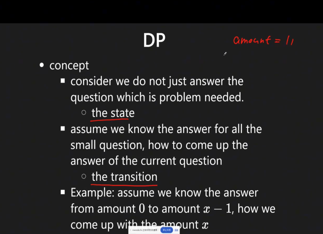
Step

Step 1. define dp def Step 2. define dp eq Step 3. check boundary condition, req, edge case Step 4. get the result

References

• Dynamic Programming Patterns
• DP Tutorial

Recognition

The constraint cues come from the ruler in complexity_cheatsheet.md.

Problem Categories

Category 1: Linear DP

• Description: Single sequence problems with linear dependencies
• Examples: LC 70 (Climbing Stairs), LC 198 (House Robber), LC 300 (LIS)
• Pattern: dp[i] depends on dp[i-1], dp[i-2], etc.
• Sub-shape — prefix partition: dp[i] instead scans every cut point j < i and tests the whole segment s[j:i] — LC 139 (Word Break), LC 132, LC 279. See Template 1b.
• Sub-shape — value-keyed (DP + hash map): the only legal predecessor of x is one known value (x - d), so dp lives in a map keyed by value and the inner loop disappears — LC 1218. See Template 7a.

Category 2: Grid/2D DP

• Description: Problems on 2D grids or matrices
• Examples: LC 62 (Unique Paths), LC 64 (Minimum Path Sum), LC 221 (Maximal Square)
• Pattern: dp[i][j] depends on neighbors

Category 3: Interval DP

• Description: Problems on intervals or subarrays
• Examples: LC 312 (Burst Balloons), LC 1000 (Minimum Cost to Merge Stones)
• Pattern: dp[i][j] for interval [i, j]

Category 3-2: Game Theory / Minimax DP → dp_advanced.md

• Description: Two-player optimal play on arrays; each player picks from either end
• Examples: LC 486 (Predict the Winner), LC 877 (Stone Game), LC 1140 (Stone Game II)
• Pattern: dp[i][j] = max relative score difference (current player minus opponent) on nums[i..j]
• Recurrence: dp[i][j] = max(nums[i] - dp[i+1][j], nums[j] - dp[i][j-1]) — derivation and template in dp_advanced.md

Category 4: Tree DP

• Description: DP on tree structures

• Examples: LC 337 (House Robber III), LC 968 (Binary Tree Cameras)

• Pattern: State at each node depends on children

• 📚 Implementation: Tree DP problems use DFS traversal for implementation. See dfs.md Template 6 (Bottom-up DFS) for the DFS traversal patterns used in tree DP solutions

• Sub-patterns: bottom-up (post-order) tree DP and re-rooting DP (two-pass DFS) — both in dp_advanced.md

Category 5: State Machine DP

• Description: Problems with multiple states and transitions

• Examples: LC 714 (Stock with Fee), LC 309 (Stock with Cooldown), LC 122 (Stock II)

• Pattern: Multiple DP arrays for different states

• Key Characteristic: State transitions depend on previous state + action constraints

• Sub-patterns: 2-state (LC 122), 3-state with cooldown (LC 309), 2k-state for k transactions (LC 123 / 188) — all in stock_trading.md

Category 6: Knapsack DP

• Description: Selection problems with constraints
• Examples: LC 416 (Partition Equal Subset), LC 494 (Target Sum)
• Pattern: dp[i][j] for items and capacity/target

Category 7: String DP

• Description: String matching, transformation, and subsequence problems
• Examples: LC 72 (Edit Distance), LC 1143 (LCS), LC 5 (Longest Palindromic Substring)
• Pattern: dp[i][j] for positions in two strings

Category 8: State Compression DP

• Description: Use bitmask to represent states, optimize space complexity
• Examples: LC 691 (Stickers to Spell Word), LC 847 (Shortest Path Visiting All Nodes)
• Pattern: dp[mask] where mask represents visited/selected items

Category 9: Monotonic Stack + DP → dp_monotonic_stack.md

Signal: a brute-force that removes elements round by round (each element is deleted once a bigger element reaches it), or an area/rectangle question over a histogram. Both are O(n^2) if simulated and O(n) with a monotonic stack that carries a DP value.

dp_monotonic_stack.md covers, in full: the survival-round transition with a worked trace, the LC 2289 template in Java and Python, the histogram area DP, the maximal square recurrence, and the LC 926 one-pass DP.

Templates & Algorithms

Template Comparison Table

Template 1: 1-D Linear DP — LC 53 ★★★★★Priority 5 of 5 — Must know — expect it in almost every loop

Recognise — one array, and the answer at position i depends only on a fixed number of earlier positions: “maximum sum of a contiguous subarray”, “number of ways to reach step n”, “cannot take two adjacent”. n ≤ 10⁵ → one O(n) pass is expected.

Key point — dp[i] is a claim about the subarray that ends exactly at i, so it has only two choices: extend the best run ending at i-1, or restart at i. The answer can end anywhere, so it is max(dp), not dp[n-1].

• State: dp[i] = best sum of a subarray ending exactly at index i
• Recurrence: dp[i] = max(nums[i], dp[i-1] + nums[i])
• Base: dp[0] = nums[0]
• Order: i ascending — dp[i] reads only dp[i-1]
• Answer: max(dp)

# python
# IDEA: dp[i] = best sum of a subarray that ENDS at i: extend the previous run or restart at i
# time = O(n), space = O(n)
# LC 53 - Maximum Subarray
def maxSubArray(nums):
    n = len(nums)
    if n == 0:
        return 0

    # State: dp[i] = max sum of a subarray ending exactly at index i
    dp = [0] * n
    dp[0] = nums[0]

    for i in range(1, n):
        # Transition: extend the run ending at i-1, or start a new run at i
        dp[i] = max(nums[i], dp[i - 1] + nums[i])

    # The answer can end anywhere, so it is the best dp[i], not dp[n-1]
    return max(dp)

// java
// LC 53 - Maximum Subarray
// IDEA: dp[i] = best sum of a subarray that ENDS at i: extend the previous run or restart at i
// time = O(n), space = O(n)
public int maxSubArray(int[] nums) {
    int n = nums.length;
    int[] dp = new int[n];
    dp[0] = nums[0];
    int best = dp[0];

    for (int i = 1; i < n; i++) {
        // extend the run ending at i-1, or start a new run at i
        dp[i] = Math.max(nums[i], dp[i - 1] + nums[i]);
        best = Math.max(best, dp[i]);   // the answer can end at any index
    }
    return best;
}

Complexity

• Time O(n): the single for i in range(1, n) loop does O(1) work per index.
• Space O(n): the dp array. dp[i] reads only dp[i-1], so one running variable makes it O(1) — that is Kadane’s algorithm.

Dry run

nums = [-2, 1, -3, 4, -1, 2]
i=0  dp=-2                       best=-2
i=1  max(1, -2+1=-1)  -> 1       best=1
i=2  max(-3, 1-3=-2)  -> -2      best=1
i=3  max(4, -2+4=2)   -> 4       restart at 4
i=4  max(-1, 4-1=3)   -> 3
i=5  max(2, 3+2=5)    -> 5       best=5   ([4, -1, 2])

Traps

• dp[i] = max(dp[i-1], nums[i]) drops the + nums[i] and returns the largest element, not the largest sum: [1, 2] gives 2 instead of 3.
• Returning dp[n-1] assumes the best run ends at the last index: [5, -9] returns -4, not 5.
• Seeding best = 0 (or dp with zeros) is wrong when every value is negative: [-3, -1] must return -1.

Not this if — the predecessor can be any earlier index, not just i-1 → LIS (Template 7). A product instead of a sum needs both the max and the min ending at i → LC 152 in kadane_algorithm.md.

Drill — LC 53 ⭐ · LC 746 (min instead of max, two steps back) · LC 152 ⭐ (carry max and min) · LC 918 (circular: total − min subarray) · LC 1191 (repeated array)

Recurrence catalogue (1-D)

Maximum subarray (Kadane) → kadane_algorithm.md

dp[i] = max(nums[i], dp[i-1] + nums[i]) is the same 1-D shape with a “restart or extend” choice, so it needs no table at all. kadane_algorithm.md covers that family in full — LC 53, LC 152 (max product), LC 918 (circular), LC 1191 (repeated array) — including index tracking and the divide-and-conquer variant.

Template 1a: Length-Indexed Table (n + 1 Slots) — LC 70

Recognise — the answer is about the first i items or a target of size i, and size 0 has a meaningful answer of its own: “number of ways to reach step n”, “can the first i characters be …”, “fewest coins to make amount a”. The tell is a base case for nothing.

Key point — dp[i] is a claim about a length (or amount), not about the element at index i. Slot 0 holds the empty prefix, so the table has n + 1 slots, the element decided at step i is nums[i-1], and the answer is dp[n].

• State: dp[i] = number of distinct ways to stand on step i
• Recurrence: dp[i] = dp[i-1] + dp[i-2] — the last move was one step or two
• Base: dp[0] = 1 (one way to stand still), dp[1] = 1
• Order: i ascending, 2 → n
• Answer: dp[n]

# python
# LC 70 - Climbing Stairs
# IDEA: dp[i] = ways to reach step i; i is a COUNT of steps, so the table has n + 1 slots
# time = O(n), space = O(n)
def climbStairs(n):
    dp = [0] * (n + 1)      # dp[0] .. dp[n]: step n is the goal, so it needs a slot
    dp[0] = 1               # one way to be at the bottom: take no step
    dp[1] = 1
    for i in range(2, n + 1):
        dp[i] = dp[i - 1] + dp[i - 2]   # last move was 1 step or 2 steps
    return dp[n]

// java
// LC 70 - Climbing Stairs
// IDEA: dp[i] = ways to reach step i; i is a COUNT of steps, so the table has n + 1 slots
// time = O(n), space = O(n)
public int climbStairs(int n) {
    int[] dp = new int[n + 1];
    dp[0] = 1;              // one way to be at the bottom: take no step
    dp[1] = 1;
    for (int i = 2; i <= n; i++) {
        dp[i] = dp[i - 1] + dp[i - 2];
    }
    return dp[n];
}

Complexity

• Time O(n): one pass of for i in range(2, n + 1), O(1) per step.
• Space O(n): the n + 1 table. Two rolling variables make it O(1) (Template 6).

Traps

• The three tells must agree — [0] * (n + 1), range(1, n + 1), return dp[n]. Mix the length view with the index view and you read s[n] off the end, or skip the last element.
• s[i-1] in a length-indexed loop is the current character, not the previous one (below).
• Seeding dp[2] without a guard: n = 1 gives a table of 2 slots and dp[2] = … raises IndexError. Seeding dp[0] and dp[1] only needs n ≥ 1.

Not this if — dp[i] is about the element at index i (“subarray ending at i”) → size n and Template 1. A whole segment s[j:i] is tested at each step → Template 1b.

Drill — LC 70 ⭐ · LC 746 (dp[n] is the “top”, one past the last step) · LC 198 ⭐ (n + 1 form below) · LC 91 ⭐ (dp[0] = 1, read s[i-1] and s[i-2:i]) · LC 926 (the s[i-1] trap)

Why two sizes exist at all — the difference comes down to what a single index in your DP array represents. Two reasons cover almost every problem; the third — physical “steps” vs “goals”, LC 746 — is in dp_advanced.md.

1. “Indices” vs “Count” (The Offset)

This is the most frequent reason for the difference.

• Loop to n (Array size = n): You are treating the index as a specific element in the input array

  • dp[i] means “the best result using the i-th element”
  • Example: dp[3] represents “result at element index 3”

• Loop to n+1 (Array size = n+1): You are treating the index as a quantity or length

  • dp[i] means “the best result using the first i elements”
  • Example: dp[3] represents “result using first 3 elements”

Example: LC 198 (House Robber)

# python
# LC 198 - House Robber, sized both ways
# IDEA: index view (dp[i] = best using house i) vs length view (dp[i] = best over the first i houses)
# time = O(n), space = O(n)
# Approach 1: Array size = n (index-based)
def rob_v1(nums):
    n = len(nums)
    if n == 0: return 0
    if n == 1: return nums[0]

    dp = [0] * n
    dp[0] = nums[0]
    dp[1] = max(nums[0], nums[1])

    for i in range(2, n):  # Loop to n
        dp[i] = max(dp[i-1], dp[i-2] + nums[i])

    return dp[n-1]  # Answer at last index

# Approach 2: Array size = n+1 (count-based)
def rob_v2(nums):
    n = len(nums)
    dp = [0] * (n + 1)  # Extra space for "0 houses"
    dp[0] = 0  # Robbing 0 houses = 0
    dp[1] = nums[0] if n > 0 else 0

    for i in range(2, n + 1):  # Loop to n+1
        dp[i] = max(dp[i-1], dp[i-2] + nums[i-1])  # Note: nums[i-1]

    return dp[n]  # Answer at position n

The s[i-1] trap — it is the current character, not the previous one

Once the table is n+1 long, i stops being a position and becomes a length. That single change is what makes s[i-1] read wrong at first glance: the -1 looks like “step back one character”, but it is only the conversion from a length to the index of that length’s last character.

dp[i]  = a claim about the FIRST i CHARACTERS  ->  i is a LENGTH (0 .. n)
s[j]   = the character sitting AT position j   ->  j is an INDEX  (0 .. n-1)

a prefix of length i ends at index i-1
        -> s[i-1] is the newest character inside dp[i]  ->  the CURRENT one

Line the two rows up once and the confusion goes away — they are off by one by construction, because the length row carries an extra “empty prefix” slot at the front:

s        =        0     1     0          (n = 3)
index    =        0     1     2          <- s is indexed 0..n-1
                  ^     ^     ^
dp slot  =  0     1     2     3          <- dp has n+1 slots
            |     |     |     |
           ""    "0"   "01"  "010"       <- the prefix dp[i] talks about

s[i-1] is never the previous character — the previous character is s[i-2], and you almost never need it, because everything already decided about it is folded into dp[i-1].

LC 926 (Flip String to Monotone Increasing) written in this view — dp[i] = min flips to make the first i characters monotone increasing:

# python
# LC 926 - Flip String to Monotone Increasing
# IDEA: dp[i] = min flips over the PREFIX OF LENGTH i, so the char decided at step i is s[i-1]
# time = O(n), space = O(n)
def minFlipsMonoIncr(s):
    n = len(s)
    dp = [0] * (n + 1)          # n+1 slots: dp[0] = empty prefix = 0 flips
    one_so_far = 0              # '1's seen so far in s[:i-1]

    for i in range(1, n + 1):   # i = prefix LENGTH, not a position
        val = s[i - 1]          # the character being decided right now

        if val == '0':
            # flip every earlier '1' -> one_so_far
            # flip this '0' to '1'   -> 1 more than dp[i-1]
            dp[i] = min(one_so_far, dp[i - 1] + 1)
        else:
            dp[i] = dp[i - 1]   # a '1' at the end is always safe, costs nothing
            one_so_far += 1

    return dp[n]                # dp[n], NOT dp[n-1]

Trace on s = "010":

i=1  val=s[0]='0'  dp[1]=min(one_so_far=0, dp[0]+1=1) = 0
i=2  val=s[1]='1'  dp[2]=dp[1]=0                 one_so_far -> 1
i=3  val=s[2]='0'  dp[3]=min(one_so_far=1, dp[2]+1=1) = 1
answer = dp[3] = 1     ("010" -> "011" or "000")

Three tells put you in the length view, and all three must agree — dp = [0] * (n + 1), for i in range(1, n + 1), return dp[n]. Mix one of them with the index view and you either read s[n] off the end of the string or silently skip its last character.

2. Handling the “Empty” Base Case

Many DP problems need a base case representing “nothing” (target sum = 0, empty string, etc.).

Examples:

• Knapsack/Coin Change: Need dp[target + 1] because dp[0] represents sum = 0
• Longest Common Subsequence: Use (n+1) x (m+1) matrix where first row/column = empty string — but a 2-D table indexed by real positions (LC 647’s dp[i][j] = s[i..j]) is n × n; see Sizing the table

# python
# LC 322 - Coin Change
# IDEA: dp[a] = fewest coins for amount a; dp[0] = 0 is the "empty" amount, so amount + 1 slots
# time = O(amount * len(coins)), space = O(amount)
def coinChange(coins, amount):
    dp = [float('inf')] * (amount + 1)  # Need amount+1
    dp[0] = 0  # Base case: 0 coins needed for amount 0

    for i in range(1, amount + 1):  # Loop to amount+1
        for coin in coins:
            if i >= coin:
                dp[i] = min(dp[i], dp[i - coin] + 1)

    return dp[amount] if dp[amount] != float('inf') else -1

Comparison Summary

Template 1b: Prefix Partition DP — LC 139 ★★★★☆Priority 4 of 5 — High value — a gap here costs you rounds

Template 1a’s n+1 sizing exists for exactly this shape. dp[i] is a claim about a prefix length, never about “the character at index i” — and this is the one 1-D family whose transition inspects a whole segment s[j:i] instead of a fixed offset like dp[i-1] or dp[i-2]. Everything else in the family swaps out one thing: the test applied to that segment.

Recognise — “can the string be segmented / broken / cut into pieces that each satisfy …”, “minimum number of cuts”, “fewest pieces”. n ≤ 300 (LC 139) → an O(n²) cut loop is fine; a dictionary of short words (L ≤ 20) lets the inner loop stop after L steps.

Key point — guess the last word. If s[:i] splits at all, the split ends with one final word s[j:i], and everything before it is the smaller problem s[:j] that dp[j] has already answered. So dp[i] is an OR over every cut point j of dp[j] AND s[j:i] in words.

        j                 i
s:  [ ---- dp[j] ---- ][ s[j:i] ]
      already solved     one word?

dp[i] is true the moment some j answers yes to both — which is why the inner loop can break on the first hit. Read i as a boundary, not a character: it is the frontier between “already segmented” and “not yet looked at”, so it legitimately reaches n — one past the last character. That is the same frontier the BFS formulation queues up.

# python
# IDEA: PREFIX PARTITION DP — dp[i] = can s[:i] be cut into dictionary words
# LC 139 - Word Break
# time = O(n^2) cuts * O(L) slice+hash, space = O(n + dictionary)
class Solution(object):
    def wordBreak(self, s, wordDict):
        n = len(s)
        words = set(wordDict)          # set, not list — see the trap below

        dp = [False] * (n + 1)         # n+1 slots, indexed by prefix LENGTH
        dp[0] = True                   # the empty prefix is always segmentable

        for i in range(1, n + 1):      # i = end boundary of the prefix
            for j in range(i):         # j = start of the candidate last word
                if dp[j] and s[j:i] in words:
                    dp[i] = True
                    break              # one valid cut is enough — it is an OR
        return dp[n]

// java
// IDEA: PREFIX PARTITION DP — dp[i] = can s[:i] be cut into dictionary words
// LC 139 - Word Break
// time = O(n^2) cuts * O(L) substring+hash, space = O(n + dictionary)
public boolean wordBreak(String s, List<String> wordDict) {
    int n = s.length();
    Set<String> words = new HashSet<>(wordDict);

    boolean[] dp = new boolean[n + 1];   // n+1 slots, indexed by prefix LENGTH
    dp[0] = true;                        // the empty prefix is always segmentable

    for (int i = 1; i <= n; i++) {       // i = end boundary of the prefix
        for (int j = 0; j < i; j++) {    // j = start of the candidate last word
            if (dp[j] && words.contains(s.substring(j, i))) {
                dp[i] = true;
                break;                   // one valid cut is enough — it is an OR
            }
        }
    }
    return dp[n];
}

Complexity — stated honestly. The doubled for i / for j loop is O(n²) iterations, but each one builds and hashes a substring of length up to n:

Space is O(n) for dp plus the word set. A last word longer than the longest dictionary entry can never match, so the inner loop only needs to reach back L characters:

# python
# IDEA: same DP, inner loop capped by the longest word — O(n * L^2), effectively linear in n
# time = O(n * L^2), space = O(n)
L = max(map(len, words))
for i in range(1, n + 1):
    for j in range(max(0, i - L), i):
        if dp[j] and s[j:i] in words:
            dp[i] = True
            break

A second solution, kept because it is a different algorithm: treat each boundary i as a graph node and each dictionary word s[i:j] as an edge i → j, then ask whether n is reachable. Same bound, but it only expands boundaries that are actually reachable, and it is the form to reach for when the interviewer frames the problem as a path search.

# python
# IDEA: BFS over boundaries — from boundary i, every dictionary word s[i:j] reaches boundary j
# time = O(n * L) cuts * O(L) slice+hash = O(n * L^2), L = longest word; space = O(n)
from collections import deque

def wordBreak(s, wordDict):
    words = set(wordDict)
    longest = max(len(w) for w in words)
    n = len(s)
    seen = [False] * (n + 1)           # boundary already queued
    seen[0] = True
    queue = deque([0])
    while queue:
        i = queue.popleft()
        if i == n:                     # the whole string is cut into words
            return True
        for j in range(i + 1, min(n, i + longest) + 1):   # no word is longer: never slice past it
            if not seen[j] and s[i:j] in words:
                seen[j] = True
                queue.append(j)
    return False

Dry run

s = "leetcode", dict = {"leet", "code"}

i=0                     dp[0] = True   (base: empty prefix)
i=1..3   no j works     dp[1..3] = False
i=4      j=0: dp[0] AND "leet" in dict  -> dp[4] = True
i=5..7   no j works     dp[5..7] = False
i=8      j=4: dp[4] AND "code" in dict  -> dp[8] = True
                                           ^ answer = dp[n] = dp[8]

Traps

• in wordDict on the raw list. s[j:i] in wordDict against a list is a linear scan with a string compare at each step — O(k·L) per lookup, so the whole solve degrades to O(n²·k·L) and TLEs. set(wordDict) makes it one hash. This is the single most common reason a correct-looking Word Break times out.
• Looping over the dictionary instead of over the cut points. The inner loop is range(i) — positions — not for w in wordDict. A word-driven inner loop is fine (it still reads only finished cells); a word-driven outer loop is not, and it silently fails the problem’s own Example 2 — "applepenapple" needs "apple" on both sides of "pen", and one pass per word can only place a word once. Why, and all five orders side by side: dp_loop_order.md.
• Returning dp[-1] after mis-sizing. With n slots instead of n+1 there is nowhere to put the dp[0] = True base case, and every answer collapses to False.

Not this if — the problem wants every split, not whether one exists: LC 131 Palindrome Partitioning is backtracking, because DP prunes to a yes/no or an optimum and cannot enumerate exponentially many outputs any faster. LC 140 is the hybrid: DP to prove a split exists, then backtracking to list them.

Drill — LC 139 ⭐ · LC 91 ⭐ (segment capped at 2 digits, combine = sum) · LC 279 (segment = a perfect square, combine = min + 1) · LC 132 (palindrome test, min cuts) · LC 140 (collect sentences) · LC 472 (the dictionary is the input itself)

Similar LeetCode Problems

Every one of these is the same dp[i] = f(dp[j], segment(j, i)) skeleton. Only the segment test and the combining operator change:

Template 2: 2-D Grid DP — LC 64 ★★★★★Priority 5 of 5 — Must know — expect it in almost every loop

Recognise — a grid is handed to you and movement is only right / down (or any one-way direction): “minimum path sum from top-left to bottom-right”, “number of unique paths”, “largest square of 1s”. m, n ≤ 200 → O(m·n) is expected.

Key point — a one-way move makes the grid a DAG: the best path to (i, j) must have come from above or left, and row-major order fills both before (i, j). So each cell is computed once, and no visited set is needed.

# python
# LC 64 - Minimum Path Sum
# IDEA: a cell is reached from above or from the left, so take the cheaper and add the cell
# time = O(m * n), space = O(m * n)
def minPathSum(grid):
    m, n = len(grid), len(grid[0])
    dp = [[0] * n for _ in range(m)]
    dp[0][0] = grid[0][0]

    for i in range(1, m):                 # first column: only from above
        dp[i][0] = dp[i - 1][0] + grid[i][0]
    for j in range(1, n):                 # first row: only from the left
        dp[0][j] = dp[0][j - 1] + grid[0][j]

    for i in range(1, m):
        for j in range(1, n):
            dp[i][j] = grid[i][j] + min(dp[i - 1][j], dp[i][j - 1])

    return dp[m - 1][n - 1]

// java
// LC 64 - Minimum Path Sum
// IDEA: a cell is reached from above or from the left, so take the cheaper and add the cell
// time = O(m * n), space = O(m * n)
public int minPathSum(int[][] grid) {
    int m = grid.length;
    int n = grid[0].length;
    int[][] dp = new int[m][n];

    dp[0][0] = grid[0][0];                       // base: starting cell
    for (int i = 1; i < m; i++) {                // first column — only from above
        dp[i][0] = dp[i - 1][0] + grid[i][0];
    }
    for (int j = 1; j < n; j++) {                // first row — only from the left
        dp[0][j] = dp[0][j - 1] + grid[0][j];
    }

    for (int i = 1; i < m; i++) {                // the rest: min of above vs left
        for (int j = 1; j < n; j++) {
            dp[i][j] = grid[i][j] + Math.min(dp[i - 1][j], dp[i][j - 1]);
        }
    }
    return dp[m - 1][n - 1];
}

Complexity

• Time O(m·n): the nested for i / for j visits each cell once, O(1) per cell.
• Space O(m·n): the dp table. Row i reads only row i-1, so one row of length n is enough — O(n).

Dry run

grid          dp
1 3 1         1  4  5
1 5 1    ->   2  7  6
4 2 1         6  8  7     answer dp[2][2] = 7   (1 → 3 → 1 → 1 → 1)

Traps

• Filling the first row / column with the general formula reads dp[-1][j], which in Python is the last row, not an error: the answer is silently wrong. Seed them separately.
• grid = [[5]] (1 × 1): both seeding loops are empty and the answer is grid[0][0]; a solution that starts with dp[1][1] indexes out of range.
• LC 63 (obstacles): an obstacle in the first row blocks every cell to its right, so the first-row seed is not 1 everywhere.

Not this if — movement in all four directions makes cycles, so “already filled” stops being true → Dijkstra (LC 1631, table below). Two strings instead of one grid → the table is invented, not handed to you → Template 2a.

Drill — LC 64 · LC 62 ⭐ (count instead of min) · LC 63 (obstacles in the seed row) · LC 120 (triangle, bottom-up) · LC 221 (1 + min of three neighbours) · LC 174 (fill from the bottom-right)

DP or Dijkstra — One-Way vs Four-Way Moves

Rule: If movement is constrained to one direction (right/down) → use 2D DP. If all 4 directions are allowed → use Dijkstra (or BFS with priority).

Recurrence catalogue (2-D)

The Python transcription, the in-place variant, the O(m) rolling-row form, the top-down memoised form, the four-approach comparison table, the similar-problem map and the [[1,3,1],[1,5,1],[4,2,1]] trace are in dp_advanced.md; the counting twin LC 62 (Unique Paths) is worked in dp_examples.md.

Template 2a: 2-D Table Shape and Fill Order — LC 516 ★★★★★Priority 5 of 5 — Must know — expect it in almost every loop

Template 2 is the easy 2-D case: the table is the input grid, so dp[i][j] sits where the problem already put it. The other two 2-D families — interval DP (Template 3, Template 10) and two-sequence DP (Template 8, Template 9) — invent a table the problem never handed you, and there the recurrence is rarely what sinks people. The table is: what shape is it, which cells does the recurrence read, and therefore which loop order is legal. This section is the shared map; the templates below assume it.

Recognise — a 2-D table the problem did not hand you: “longest palindromic subsequence”, “minimum insertions to make a palindrome”, “edit distance / LCS between two strings”, “burst / merge everything in a range”. n ≤ 1000 → O(n²) cells; n ≤ 500 with a split point → O(n³).

Key point — every dp[...] on the right-hand side of the transition is an arrow into dp[i][j]; a loop order is legal exactly when every arrow lands on a cell that is already filled. LC 516 reads row i+1 and column j-1, so i descends and j ascends.

• State: dp[i][j] = longest palindromic subsequence inside s[i..j] (Shape A, n × n)
• Recurrence: dp[i+1][j-1] + 2 if s[i] == s[j], else max(dp[i+1][j], dp[i][j-1])
• Base: the diagonal, dp[i][i] = 1
• Order: i from n-1 down to 0, j from i+1 up to n-1
• Answer: the top-right corner, dp[0][n-1]

# python
# LC 516 - Longest Palindromic Subsequence
# IDEA: i descends so row i+1 is already done; j ascends so column j-1 is already done
# time = O(n^2), space = O(n^2)
def longestPalindromeSubseq(s):
    n = len(s)
    dp = [[0] * n for _ in range(n)]

    for i in range(n - 1, -1, -1):         # bottom row first
        dp[i][i] = 1                       # base: one character
        for j in range(i + 1, n):          # left to right, above the diagonal
            if s[i] == s[j]:
                dp[i][j] = dp[i + 1][j - 1] + 2
            else:
                dp[i][j] = max(dp[i + 1][j], dp[i][j - 1])

    return dp[0][n - 1]

// java
// LC 516 - Longest Palindromic Subsequence
// IDEA: i descends so row i+1 is already done; j ascends so column j-1 is already done
// time = O(n^2), space = O(n^2)
public int longestPalindromeSubseq(String s) {
    int n = s.length();
    int[][] dp = new int[n][n];

    for (int i = n - 1; i >= 0; i--) {         // bottom row first
        dp[i][i] = 1;                          // base: one character
        for (int j = i + 1; j < n; j++) {      // left to right, above the diagonal
            if (s.charAt(i) == s.charAt(j)) {
                dp[i][j] = dp[i + 1][j - 1] + 2;
            } else {
                dp[i][j] = Math.max(dp[i + 1][j], dp[i][j - 1]);
            }
        }
    }
    return dp[0][n - 1];
}

Complexity

• Time O(n²): the for i / for j pair visits each cell of the upper triangle once, O(1) per cell. A split point k nested inside (Template 3) makes it O(n³).
• Space O(n²): the n × n table. Shape B tables compress to one row; Shape A does not (see Space compression below).

Dry run — LC 516 on s = "bbbab" is worked cell by cell in Shape A below (Worked table — LC 516); the answer is the corner, 4.

Traps

• Filling in the wrong direction. Shape A’s i must descend; for i in range(n) reads dp[i+1][...] while it is still 0 and the answer comes out silently too small — no crash, no wrong-index exception. Derive the direction from the arrow table below instead of recalling it.
• Touching the dead triangle. In Shape A with j == i + 1, dp[i+1][j-1] is dp[i+1][i], below the diagonal. It is 0 / False by construction — which happens to be correct for LC 516 (0 + 2 = 2, a two-character palindrome) and wrong for LC 5, which is exactly why that one needs its explicit j - i <= 2 guard.
• Copying the base row from another problem. 0, i and 1 are all correct base rows for different Shape B problems — LCS, edit distance, LC 115 — see the callout under Shape B.
• Compressing before knowing you only need the number. The rolling row is free only when the answer is a value; the moment the follow-up is “and which operations?”, you need the table back.

Not this if — the grid is handed to you and i, j are coordinates → Template 2. The transition needs a split point k inside the range → only the length-driven order (Order B) is safe → Template 3.

Drill — LC 516 · LC 647 ⭐ (n × n, count the Trues) · LC 5 ⭐ (the j - i <= 2 guard) · LC 1143 ⭐ (Shape B) · LC 72 ⭐ (Shape B, three moves) · LC 1312 (min insertions)

The rule that decides the loop order

Write the transition first. Every dp[...] on its right-hand side is an arrow pointing into dp[i][j]. A loop order is legal exactly when every arrow lands on a cell that is already filled. There is nothing else to it.

That table is the whole decision procedure, and it is why LC 516’s loop runs i backwards while LC 72’s runs i forwards — not style, not taste, just which neighbours each recurrence reads.

The 1-D sibling of this table — plus the other loop-order axis, whether an item loop may sit outside the state loop at all — is dp_loop_order.md.

Which shape am I building?

What do i and j MEAN in dp[i][j]?

├── ONE sequence; i and j are the two ENDS of a sub-range s[i..j]
│      → Shape A — n × n, only the upper triangle is real,
│        base on the diagonal, answer at the TOP-RIGHT dp[0][n-1]
│        LC 516, 5, 647, 1312, 312, 877
│
├── TWO sequences; i and j are PREFIX LENGTHS (first i of s1, first j of s2)
│      → Shape B — (m+1) × (n+1), row 0 / column 0 are the empty prefixes,
│        answer at the BOTTOM-RIGHT dp[m][n]
│        LC 72, 1143, 115, 97, 10
│
└── a real grid handed to you; i and j are COORDINATES
       → Template 2 above — m × n, answer at dp[m-1][n-1]
         LC 62, 64, 221

Sizing the table — n × n or (n+1) × (n+1)?

Worked on LC 647 (Palindromic Substrings). This is Template 1a’s rule applied to two axes. The size comes from what an index means, not from how many dimensions the table has:

Memory trick: real index → n × n; “first i characters” → n + 1. The extra slot exists only to hold the empty prefix. A sub-range s[i..j] with i <= j is never empty, so Shape A has nothing to put there.

# python
# LC 647 - Palindromic Substrings
# IDEA: dp[i][j] = s[i..j] is a palindrome. i and j are REAL indexes, so n x n, not n+1.
# time = O(n^2), space = O(n^2)
def countSubstrings(s):
    n = len(s)
    dp = [[False] * n for _ in range(n)]   # n slots: every index is a character of s
    count = 0

    for length in range(1, n + 1):         # short ranges first: dp[i+1][j-1] is shorter
        for i in range(n - length + 1):
            j = i + length - 1             # j is a position too, so it stays <= n-1
            if s[i] == s[j] and (length <= 2 or dp[i + 1][j - 1]):
                dp[i][j] = True
                count += 1

    return count

Compare LC 1143 (Shape B): dp[i][j] is “first i of s1, first j of s2”, so i runs to m — one past the last index — and the table needs m + 1 rows to have somewhere to put it.

The tell is consistency, as in 1-D. Index view: [[...] * n for _ in range(n)], loops stay <= n-1, compare s[i], return dp[0][n-1]. Length view: (m+1) × (n+1), loops run 1 → m, compare s1[i-1], return dp[m][n]. Size LC 647 at n + 1 while still comparing s[i] and the code may still pass — but row n is dead weight, and the next edit that loops to n reads s[n] off the end.

Shape A — one sequence, i/j are the two ends

State: dp[i][j] = the answer for the sub-range s[i..j].

            j = 0      1        2      ...    n-1
  i = 0   [ base ] [   ?  ] [   ?  ]  ...  [ 🎯 dp[0][n-1] ]   ← the answer
      1   [ dead ] [ base ] [   ?  ]  ...  [      ?        ]
      2   [ dead ] [ dead ] [ base ]  ...  [      ?        ]
      :
    n-1   [ dead ] [ dead ] [ dead ]  ...  [    base       ]

  diagonal  i == j : the length-1 base case  (dp[i][i] = 1, or True)
  below it  i >  j : an empty range — never written, never read
  corner   (0, n-1): the whole sequence — this is what you return

Dependency — the three cells a boundary-shrinking transition reads:

   the 2 x 2 window, drawn the same way up as the table above:

                        j-1              j
                  ┌──────────────┬──────────────┐
        row i     │  dp[i][j-1]  │   dp[i][j]   │  ← 🎯 being filled
                  ├──────────────┼──────────────┤
        row i+1   │ dp[i+1][j-1] │  dp[i+1][j]  │
                  └──────────────┴──────────────┘

   dp[i][j]  ⟵  dp[i][j-1]     →  from the LEFT      — drop the right end s[j]
   dp[i][j]  ⟵  dp[i+1][j]     ↑  from BELOW         — drop the left end  s[i]
   dp[i][j]  ⟵  dp[i+1][j-1]   ↗  from BELOW-LEFT    — drop BOTH ends

   Every arrow travels UP and to the RIGHT. Nothing arrives from above or from
   the right, so the table fills from the diagonal OUTWARD, toward the
   top-right corner.

Order A — i backward, j forward (write this one)

# python
# LC 516 - Longest Palindromic Subsequence
# IDEA: i descends so row i+1 is already done; j ascends so column j-1 is already done
# time = O(n^2), space = O(n^2)
def longestPalindromeSubseq(s):
    n = len(s)
    dp = [[0] * n for _ in range(n)]

    for i in range(n):                 # base: one character is a palindrome of length 1
        dp[i][i] = 1

    for i in range(n - 1, -1, -1):     # ↑ bottom row first
        for j in range(i + 1, n):      # → left to right, staying above the diagonal
            if s[i] == s[j]:
                dp[i][j] = dp[i + 1][j - 1] + 2
            else:
                dp[i][j] = max(dp[i + 1][j], dp[i][j - 1])

    return dp[0][n - 1]

Order B — by interval length (diagonal sweep)

# python
# IDEA: same table, one diagonal at a time. The only order that works when the transition
#       needs a split point k (dp[i][k] and dp[k][j]) instead of the two ends.
# time = O(n^2) for a two-end transition, O(n^3) once a k-loop is nested inside
n = len(s)
dp = [[0] * n for _ in range(n)]
for i in range(n):
    dp[i][i] = 1                        # base: the length-1 diagonal
for length in range(2, n + 1):          # sub-range length: short → long
    for i in range(n - length + 1):     # left end
        j = i + length - 1              # right end is derived, never looped
        if s[i] == s[j]:                # same transition as Order A (LC 516)
            dp[i][j] = dp[i + 1][j - 1] + 2
        else:
            dp[i][j] = max(dp[i + 1][j], dp[i][j - 1])

Both are legal — here is the order the cells actually get filled (n = 5)

   Order A  (i: n-1→0, j: i+1→n-1)        Order B  (length: 2→n, i: 0→n-length)
          j0   j1   j2   j3   j4                  j0   j1   j2   j3   j4
    i0     ·    7    8    9   10            i0     ·    1    5    8   10
    i1          ·    4    5    6            i1          ·    2    6    9
    i2               ·    2    3            i2               ·    3    7
    i3                    ·    1            i3                    ·    4
    i4                         ·            i4                         ·

    row by row, bottom → top                diagonal by diagonal, ↗

  Check the corner cell dp[0][4] — step 10 in both orders.
  It reads dp[1][3], dp[1][4], dp[0][3]:
    Order A → steps 5, 6, 9   ✅ all filled before step 10
    Order B → steps 6, 9, 8   ✅ all filled before step 10

How to pick: Order A when the transition moves the two ends (dp[i+1][j-1], dp[i+1][j], dp[i][j-1]) — palindromes, LCS against the reverse of the same string. Order B when the transition needs a split point k strictly inside the range (dp[i][k] + dp[k][j]) — burst balloons, merge stones, matrix chain — because there “already filled” means strictly shorter, and only a length-driven loop guarantees that.

Worked table — longest palindromic subsequence on s = "bbbab"

LC 516, filled with the code above:

   s =       b    b    b    a    b
             j0   j1   j2   j3   j4
   b   i0  [ 1 ][ 2 ][ 3 ][ 3 ][ 4 ]  ← 🎯 answer = 4
   b   i1    ·  [ 1 ][ 2 ][ 2 ][ 3 ]
   b   i2    ·    ·  [ 1 ][ 1 ][ 3 ]
   a   i3    ·    ·    ·  [ 1 ][ 1 ]
   b   i4    ·    ·    ·    ·  [ 1 ]

   dp[2][3] = 1 : 'b' != 'a'      → max(dp[3][3]=1, dp[2][2]=1) = 1
   dp[0][2] = 3 : s[0]=='b'==s[2] → dp[1][1] + 2 = 3          ("bbb")
   dp[1][3] = 2 : 'b' != 'a'      → max(dp[2][3]=1, dp[1][2]=2) = 2
   dp[0][4] = 4 : s[0]=='b'==s[4] → dp[1][3] + 2 = 4          ("bbbb")

Which way did it go? — walking the table backwards

The forward pass stores values. The decisions are recovered afterwards by re-asking, at each cell, which neighbour produced that value — no parent pointers needed, just re-evaluate the transition:

   at (0,4)  s[0]=='b'==s[4]           → matched pair: take both, jump ↘ to (1,3)
   at (1,3)  'b' != 'a', and
             dp[1][2]=2 > dp[2][3]=1   → the max came from the LEFT: drop s[3], move to (1,2)
   at (1,2)  s[1]=='b'==s[2]           → matched pair: take both, jump ↘ to (2,1)
   at (2,1)  i > j                     → empty range: stop

   pairs collected, outer → inner:  (s0, s4) then (s1, s2)
   answer string:   b [ b  b ] b   =  "bbbb"   ✓ length 4 = dp[0][4]

Shape A problems

Two Shape A problems have no character test at all, and they are the ones that pick the fill order for you:

• LC 312 (Burst Balloons) — a split point, so Order B only: dp[i][j] = max over k in (i, j) of dp[i][k] + dp[k][j] + b[i]*b[k]*b[j]. Worked in Template 3.
• LC 877 / LC 486 (Stone Game / Predict the Winner) — same triangle, but dp[i][j] holds a score difference: max(nums[i] - dp[i+1][j], nums[j] - dp[i][j-1]). Two ends, so Order A. The minimax reasoning is in dp_advanced.md.

Shape B — two sequences, i/j are prefix lengths

State: dp[i][j] = the answer for the first i characters of s1 and the first j characters of s2. So the characters this cell decides about are s1[i-1] and s2[j-1] — the off-by-one everyone trips on is just a consequence of row/column 0 meaning the empty prefix.

                  ""     s2[0]  s2[1]   ...   s2[n-1]
             j =   0       1      2     ...      n
   ""    i =  0  [base] [base] [base]  ...  [ base ]   ← s1 is empty
  s1[0]       1  [base] [  ?  ][  ?  ] ...  [  ?   ]
  s1[1]       2  [base] [  ?  ][  ?  ] ...  [  ?   ]
    :
  s1[m-1]     m  [base] [  ?  ][  ?  ] ...  [ 🎯 dp[m][n] ]  ← the answer

  row 0 / column 0 : one string is empty, so the answer is FORCED, not computed
  every other cell : three neighbours, one decision

Dependency — three arrows, all arriving from above / left / above-left:

   the same 2 x 2 window, one row higher:

                        j-1              j
                  ┌──────────────┬──────────────┐
        row i-1   │ dp[i-1][j-1] │  dp[i-1][j]  │
                  ├──────────────┼──────────────┤
        row i     │  dp[i][j-1]  │   dp[i][j]   │  ← 🎯 being filled
                  └──────────────┴──────────────┘

   dp[i][j]  ⟵  dp[i-1][j-1]   ↘  from ABOVE-LEFT   — consume from BOTH strings
   dp[i][j]  ⟵  dp[i-1][j]     ↓  from ABOVE        — consume from s1 only
   dp[i][j]  ⟵  dp[i][j-1]     →  from the LEFT     — consume from s2 only

   Nothing arrives from below or from the right, so plain row-major
   (i: 1 → m, inner j: 1 → n) is legal — and it is the only order anyone writes.

What each move means — the recurrence changes per problem, the geometry never does:

# python
# LC 72 - Edit Distance
# IDEA: Shape B — base row/col are the forced answers, then row-major over three neighbours
# time = O(m * n), space = O(m * n)  → O(min(m, n)) once rolled
def minDistance(s1, s2):
    m, n = len(s1), len(s2)
    dp = [[0] * (n + 1) for _ in range(m + 1)]

    for i in range(m + 1):
        dp[i][0] = i          # s2 empty → delete every character of s1
    for j in range(n + 1):
        dp[0][j] = j          # s1 empty → insert every character of s2

    for i in range(1, m + 1):
        for j in range(1, n + 1):
            if s1[i - 1] == s2[j - 1]:
                dp[i][j] = dp[i - 1][j - 1]          # ↘ free
            else:
                dp[i][j] = 1 + min(
                    dp[i - 1][j],                    # ↓ delete
                    dp[i][j - 1],                    # → insert
                    dp[i - 1][j - 1],                # ↘ replace
                )

    return dp[m][n]

The base row is where the bug lives. dp[i][0] = i for edit distance, 0 for LCS, 1 for LC 115 — the empty string is a subsequence of anything, exactly once. Derive it, never copy it: put i = 0 into your own state sentence and read the answer off in English.

Worked table — edit distance on "horse" → "ros", with the path it chose

LC 72, filled with the code above:

              ""    r     o     s
        ""  [ 0*]   1     2     3
        h   [ 1 ] [ 1*]   2     3
        o   [ 2 ]   2   [ 1*]   2
        r   [ 3 ]   2   [ 2*]   2
        s   [ 4 ]   3     3   [ 2*]
        e   [ 5 ]   4     4   [ 3*]   ← 🎯 dp[5][3] = 3

   * = the cells on the chosen path, recovered by walking backwards from dp[5][3]:

   (5,3) 'e' vs 's' ✗   1 + min(↓ dp[4][3]=2, → dp[5][2]=4, ↘ dp[4][2]=3)
                        the min came from ↓   ⇒ DELETE 'e'
   (4,3) 's' == 's' ✓   free ↘                ⇒ KEEP 's'
   (3,2) 'r' vs 'o' ✗   1 + min(↓ dp[2][2]=1, → dp[3][1]=2, ↘ dp[2][1]=2)
                        the min came from ↓   ⇒ DELETE 'r'
   (2,2) 'o' == 'o' ✓   free ↘                ⇒ KEEP 'o'
   (1,1) 'h' vs 'r' ✗   1 + min(↓ dp[0][1]=1, → dp[1][0]=1, ↘ dp[0][0]=0)
                        the min came from ↘   ⇒ REPLACE 'h' → 'r'
   (0,0) both prefixes empty                  ⇒ stop

   replayed forwards:   replace h→r   "horse" → "rorse"
                        keep    o
                        delete  r     "rorse" → "rose"
                        keep    s
                        delete  e     "rose"  → "ros"    ✓ 3 ops = dp[5][3]

Read the path geometrically: ↘ means a character survives, ↓ means a character of s1 is spent, → means a character of s2 is spent. The identical walk over the LC 1143 table spells out the actual common subsequence instead of an operation list — same table, same backward walk, different thing recorded on the way.

Space compression — and when it is not available

dp[i][j] reads only row i and row i-1, so Shape B collapses to two rows, then to one plus a scalar for the diagonal that is about to be overwritten:

# python
# IDEA: rolling row — prev is row i-1, cur is row i. s2 is the inner axis, so pass the
#       SHORTER string as s2.
# time = O(m * n), space = O(min(m, n))
def minDistance_rolled(s1, s2):
    m, n = len(s1), len(s2)
    prev = list(range(n + 1))
    for i in range(1, m + 1):
        cur = [i] + [0] * n
        for j in range(1, n + 1):
            cur[j] = prev[j - 1] if s1[i - 1] == s2[j - 1] else 1 + min(prev[j], cur[j - 1], prev[j - 1])
        prev = cur
    return prev[n]

Shape A does not compress this way. dp[i][j] reads row i+1 at two different columns (j-1 and j), and the diagonal sweep keeps reaching back across every earlier diagonal — there is no “last two rows” window to hold. Budget O(n²) for interval DP and move on.

And do not compress at all if you need the traceback: the rolling row throws away exactly the cells the backward walk would have read. Whenever the answer is the path rather than the number, keep the full table (or store the chosen move per cell).

Shape B problems

Two more live on the same grid without a s1 vs s2 character test:

• LC 97 (Interleaving String) — boolean, and the comparison is against a third string: dp[i][j] = (dp[i-1][j] and s1[i-1] == s3[i+j-1]) or (dp[i][j-1] and s2[j-1] == s3[i+j-1]). No diagonal at all — only ↓ and →, which is the shape of “every character comes from exactly one of the two sources”.
• LC 10 (Regular Expression Matching) — the j axis is the pattern. A plain character or . is the ordinary ↘; '*' splits into “zero copies” dp[i][j-2] and “one more copy” dp[i-1][j], both of which still read only left and above, so row-major still holds.

The 2-D DP cheat sheet

Template 3: Interval DP — LC 312

The table is Shape A — n × n, upper triangle, answer in the top-right corner. Its skeleton, the two legal fill orders and why a split point forces the length-driven one are in Template 2a.

Recognise — the cost of an operation depends on neighbours that change as you go: “burst balloons, coins = left × this × right”, “merge adjacent piles, cost = their sum”, “multiply a chain of matrices”. n ≤ 300–500 → the O(n³) split-point loop is what the limit was set for.

Key point — think about which element is processed last, not first. When k is the last balloon burst inside the open interval (i, j), everything in (i, k) and (k, j) is already gone, so the two sides are independent subproblems and k’s neighbours are exactly i and j.

• State: dp[i][j] = max coins from bursting every balloon strictly between i and j
• Recurrence: dp[i][j] = max over i < k < j of dp[i][k] + dp[k][j] + b[i]·b[k]·b[j]
• Base: dp[i][i+1] = 0 — an open interval with nothing inside
• Order: interval length ascending (a split point reads strictly shorter ranges)
• Answer: dp[0][n+1], after padding b = [1] + nums + [1]

# python
# LC 312 - Burst Balloons
# IDEA: interval DP — pick k as the LAST balloon burst in (left, right); its neighbours are then fixed
# time = O(n^3), space = O(n^2)
def maxCoins(nums):
    n = len(nums)
    balloons = [1] + nums + [1]                 # boundary balloons with value 1
    dp = [[0] * (n + 2) for _ in range(n + 2)]  # dp[i][j]: open interval (i, j)

    for length in range(2, n + 2):              # short intervals first
        for left in range(n + 2 - length):
            right = left + length
            for k in range(left + 1, right):    # k = the LAST balloon burst in (left, right)
                coins = balloons[left] * balloons[k] * balloons[right]
                total = coins + dp[left][k] + dp[k][right]
                dp[left][right] = max(dp[left][right], total)

    return dp[0][n + 1]

// java
// LC 312 - Burst Balloons
// IDEA: interval DP — pick k as the LAST balloon burst in (i, j); its neighbours are then fixed
// time = O(n^3), space = O(n^2)
public int maxCoins(int[] nums) {
    int n = nums.length;
    int[] balloons = new int[n + 2];          // boundaries: [1, ...nums..., 1]
    balloons[0] = 1;
    balloons[n + 1] = 1;
    for (int i = 0; i < n; i++) {
        balloons[i + 1] = nums[i];
    }

    int[][] dp = new int[n + 2][n + 2];       // dp[i][j]: open interval (i, j)
    for (int len = 2; len <= n + 1; len++) {  // short intervals first
        for (int i = 0; i <= n + 1 - len; i++) {
            int j = i + len;
            for (int k = i + 1; k < j; k++) { // k = the LAST balloon burst in (i, j)
                int total = balloons[i] * balloons[k] * balloons[j] + dp[i][k] + dp[k][j];
                dp[i][j] = Math.max(dp[i][j], total);
            }
        }
    }
    return dp[0][n + 1];
}

Complexity

• Time O(n³): length × left is O(n²) intervals, and the for k split loop is O(n) inside each.
• Space O(n²): the (n+2) × (n+2) table. Interval DP does not roll — a split point reaches back across every shorter length.

Dry run

nums = [3, 1, 5]   ->  balloons = [1, 3, 1, 5, 1]   (indexes 0..4)

length 2: every (i, i+2) has one balloon inside
  dp[0][2] = 1*3*1 = 3     dp[1][3] = 3*1*5 = 15     dp[2][4] = 1*5*1 = 5
length 3:
  dp[0][3] = max(k=1: 1*3*5 + 0 + dp[1][3]=15 -> 30,  k=2: 1*1*5 + dp[0][2]=3 + 0 -> 8)  = 30
  dp[1][4] = max(k=2: 3*1*1 + 0 + dp[2][4]=5 -> 8,    k=3: 3*5*1 + dp[1][3]=15 + 0 -> 30) = 30
length 4:
  dp[0][4] = max(k=1: 3 + 0 + 30 = 33,  k=2: 1 + 3 + 5 = 9,  k=3: 5 + 30 + 0 = 35) = 35

Traps

• Choosing the first balloon instead of the last. Bursting k first leaves (i, k) and (k, j) as neighbours of each other, so the subproblems are not independent and no recurrence falls out.
• Looping left before length. for left … for right … reads dp[k][right] for a k > left that has not been filled yet; only an outer length loop guarantees “strictly shorter is done”.
• Forgetting the padding. Without [1] + nums + [1], the first and last balloons have no neighbour to multiply by: nums = [5] must return 5.

Not this if — the transition only moves the two ends (dp[i+1][j-1], dp[i+1][j], dp[i][j-1]) with no split point → O(n²) Shape A, Order A (Template 2a). Two players taking from the ends → minimax DP in dp_advanced.md.

Drill — LC 312 · LC 1039 (polygon triangulation, same split loop) · LC 1547 (cut a stick: sort the cuts, pad the ends) · LC 664 (strange printer) · LC 1000 (merge k stones) · LC 546 (remove boxes, a third state)

The inclusive-boundary variant, the top-down memoised form, the worked nums = [3,1,5,8] trace, the recognition checklist, the common mistakes, the O(n³)/O(n²) derivation, the abstract split-point / matrix-chain skeletons and the backward-i + forward-j loop-order rule are in dp_advanced.md.

Template 4: 0/1 Knapsack — LC 416 ★★★★★Priority 5 of 5 — Must know — expect it in almost every loop

The knapsack family — LC 416 itself, the subset-sum reduction, unbounded, bounded and group knapsack, and the loop-order rule — is worked in knapsack.md; a Traditional Chinese walkthrough of the 0/1 case is knapsack_01_zh.md. What follows is the shape worth memorising.

Recognise — each element is used at most once, and you are choosing a subset against a budget or a target: “partition into two subsets with equal sum”, “assign + or − to reach target”, “minimise the difference between two groups”, “choose items within a capacity”. The target is small (sum ≤ 10⁴–2·10⁴) → an O(n · target) table is expected.

Key point — with one 1-D array, iterate the capacity backward: when dp[w] is updated for an item, dp[w - weight] has not been touched yet in this pass, so it still means “without this item”, and each item is counted at most once.

• State: dp[w] = the best value of a subset of the items seen so far with total weight ≤ w
• Recurrence: dp[w] = max(dp[w], dp[w - weight] + value) — skip the item, or take it
• Base: dp[*] = 0 — the empty subset
• Order: items outer; capacity inner, backward from capacity to weight
• Answer: dp[capacity]

# python
# IDEA: 0/1 knapsack, max value — dp[w] = best value within capacity w; the backward loop uses each item once
# time = O(n * W), space = O(W)
def knapsack_01(weights, values, capacity):
    dp = [0] * (capacity + 1)                 # dp[w] = best value with total weight <= w
    for i in range(len(weights)):
        for w in range(capacity, weights[i] - 1, -1):   # backward: dp[w - weight] is still "without i"
            dp[w] = max(dp[w], dp[w - weights[i]] + values[i])
    return dp[capacity]

// java
// IDEA: 0/1 knapsack, max value — dp[w] = best value within capacity w; the backward loop uses each item once
// time = O(n * W), space = O(W)
public int knapsack01(int[] weights, int[] values, int capacity) {
    int[] dp = new int[capacity + 1];             // dp[w] = best value with total weight <= w
    for (int i = 0; i < weights.length; i++) {
        for (int w = capacity; w >= weights[i]; w--) {   // backward: dp[w - weight] is still "without i"
            dp[w] = Math.max(dp[w], dp[w - weights[i]] + values[i]);
        }
    }
    return dp[capacity];
}

The same loop answers three questions; only the transition changes — or for “can some subset reach w” (LC 416), += for “how many subsets” (LC 494), max(…, + value) for the best value.

Complexity

• Time O(n · W): the outer loop runs n times and the backward inner loop at most W times.
• Space O(W): one row. The 2-D form dp[i][w] is O(n · W); the backward loop is what lets row i overwrite row i-1 in place.

Dry run — why the inner loop must go backward, with one item of weight 3 and value 5, capacity = 6 (the answer is 5: the item can be taken once):

dp = [0, 0, 0, 0, 0, 0, 0]
      0  1  2  3  4  5  6

Forward (WRONG):   w=3: dp[3] = dp[0] + 5 = 5
                   w=6: dp[6] = dp[3] + 5 = 10   <- dp[3] already holds this item: taken twice ❌
Backward (RIGHT):  w=6: dp[6] = dp[3] + 5 = 5    <- dp[3] is still 0, "without the item"
                   w=3: dp[3] = dp[0] + 5 = 5
                   result dp[6] = 5 ✓

Traps

• Forward inner loop. It turns 0/1 into unbounded knapsack: the single item above is taken twice.
• Inner loop running below the weight. range(capacity, -1, -1) reads dp[w - weight] at a negative index, which in Python is the end of the array, not an error.
• The wrong transition for the question. Using or on a count table loses the number of ways. On a boolean table, max equals or, but or makes the intent clearer.

Not this if — an item may be reused (coins, unlimited supply) → unbounded knapsack, inner loop forward, and the loop nesting depends on whether order matters → knapsack.md. Values are huge but n ≤ 20 → enumerate subsets / meet in the middle instead of a sum table.

Drill — LC 416 ⭐ · LC 494 (count subsets: (total + target) / 2) · LC 1049 (largest reachable sum ≤ total / 2) · LC 474 (two capacities, both backward) · LC 879 (count, 2-D capacity) — all in knapsack.md.

Template 5: State Machine DP — LC 309

The whole LC 121/122/123/188/309/714 family — every variant, every state count — is worked in stock_trading.md. What follows is the shape worth memorising.

Recognise — at each step you are in one of a few named situations, and a rule says which moves are legal from each: “after you sell, you cannot buy the next day”, “at most k transactions”, “pay a fee per sale”. n ≤ 5000–10⁵ → O(n · states).

Key point — keep one variable per state, holding the best profit ending today in that state. Every transition reads only yesterday’s values, so save them before overwriting.

• State: hold (own a share), sold (sold today, so tomorrow is cooldown), rest (no share, free to buy)
• Recurrence: hold = max(hold, rest - p), sold = hold + p, rest = max(rest, sold) — all from yesterday’s values
• Base: day 0 — hold = -prices[0], sold = 0, rest = 0
• Order: days ascending
• Answer: max(sold, rest) — never end holding a share

# python
# LC 309 - Best Time to Buy and Sell Stock with Cooldown
# IDEA: three states per day; each reads yesterday's values, so snapshot before updating
# time = O(n), space = O(1)
def maxProfit(prices):
    if not prices:
        return 0
    hold = -prices[0]      # bought on day 0
    sold = 0               # cannot have sold on day 0; 0 is the neutral value
    rest = 0               # no share, not in cooldown

    for i in range(1, len(prices)):
        prev_hold, prev_sold, prev_rest = hold, sold, rest
        hold = max(prev_hold, prev_rest - prices[i])   # keep holding, or buy (only from rest)
        sold = prev_hold + prices[i]                   # sell what you held
        rest = max(prev_rest, prev_sold)               # stay idle, or finish the cooldown

    return max(sold, rest)

// java
// LC 309 - Best Time to Buy and Sell Stock with Cooldown
// IDEA: three states per day; each reads yesterday's values, so snapshot before updating
// time = O(n), space = O(1)
public int maxProfit(int[] prices) {
    if (prices.length == 0) {
        return 0;
    }
    int hold = -prices[0];
    int sold = 0;
    int rest = 0;

    for (int i = 1; i < prices.length; i++) {
        int prevHold = hold, prevSold = sold, prevRest = rest;
        hold = Math.max(prevHold, prevRest - prices[i]);  // keep holding, or buy (only from rest)
        sold = prevHold + prices[i];                      // sell what you held
        rest = Math.max(prevRest, prevSold);              // stay idle, or finish the cooldown
    }
    return Math.max(sold, rest);
}

Complexity

• Time O(n): one pass over prices; three O(1) updates per day.
• Space O(1): three state variables (and their snapshots). With k transactions it is O(k).

Dry run

prices = [1, 2, 3, 0, 2]
day 0  p=1  hold=-1  sold=0   rest=0
day 1  p=2  hold=-1  sold=1   rest=0
day 2  p=3  hold=-1  sold=2   rest=1
day 3  p=0  hold= 1  sold=-1  rest=2     buy at 0, from rest (the day-1 sale has cooled down)
day 4  p=2  hold= 1  sold=3   rest=2     answer max(3, 2) = 3

Traps

• Updating in place without snapshots. hold = max(hold, rest - p) followed by sold = hold + p sells the share bought today: on [1, 2, 3, 0, 2] the answer becomes wrong.
• Buying from sold. hold = max(hold, sold - p) skips the cooldown day; buy only from rest.
• LC 121 (one transaction) is not this code with rest = 0: there the buy must start from profit 0 every time, hold = max(hold, -p), or a second transaction sneaks in.

Not this if — no cooldown, unlimited transactions, no fee (LC 122) → greedy: sum every positive day-to-day difference. “At most k transactions” → 2k states, in stock_trading.md.

Drill — LC 309 ⭐ · LC 121 ⭐ (two states, buy from 0) · LC 122 (two states) · LC 714 (fee on sell) · LC 123 (four states) · LC 188 (2k states)

Template 6: Memoization → Tabulation → Rolling Variables — LC 198 ★★★★★Priority 5 of 5 — Must know — expect it in almost every loop

The space-optimisation ladder: write the recursion, cache it, flip it to a table, then collapse the table to k variables. recursion_to_dp.md walks the first two rungs in detail.

Recognise — a 1-D recurrence that reads a fixed window of earlier answers (dp[i-1], dp[i-2], …): “rob houses, no two adjacent”, “climb 1 or 2 steps”, “decode a digit string”. The follow-up “can you do it in O(1) space?” is the cue for the last rung.

Key point — if dp[i] reads only the last k cells, only k variables are alive. Keep the invariant p1 = dp[i-2], p2 = dp[i-1] true at the top of every iteration, and the answer is the newest rolling variable — which is valid even when the loop runs zero times.

• State: dp[i] = most money robbed from houses 0..i
• Recurrence: dp[i] = max(dp[i-1], dp[i-2] + nums[i]) — skip house i, or rob it
• Base: dp[0] = nums[0], dp[1] = max(nums[0], nums[1])
• Order: i ascending; two variables replace the table
• Answer: p2 (= dp[n-1]), never the loop temporary

# python
# LC 198 - House Robber
# IDEA: dp[i] = max(dp[i-1], dp[i-2] + nums[i]) -> only 2 vars needed
# time = O(n), space = O(1)
def rob(nums):
    if not nums:
        return 0
    n = len(nums)
    if n == 1:
        return nums[0]          # p2's seed reads nums[1], so n == 1 must leave early

    # invariant at the top of iteration i:  p1 = dp[i-2],  p2 = dp[i-1]
    p1 = nums[0]                        # dp[0]
    p2 = max(nums[0], nums[1])          # dp[1]

    for i in range(2, n):
        cur = max(p1 + nums[i], p2)     # dp[i]
        p1 = p2                         # oldest -> newest
        p2 = cur

    return p2                           # NOT `cur`

// java
// LC 198 - House Robber
// IDEA: same 2-variable rolling window; return the rolling var, not the temp
// time = O(n), space = O(1)
public int rob(int[] nums) {
    if (nums == null || nums.length == 0) return 0;
    int n = nums.length;
    if (n == 1) return nums[0];

    int p1 = nums[0];                       // dp[0]
    int p2 = Math.max(nums[0], nums[1]);    // dp[1]

    for (int i = 2; i < n; i++) {
        int cur = Math.max(p1 + nums[i], p2);
        p1 = p2;
        p2 = cur;
    }
    return p2;   // hoisting `cur` out of the loop just to return it would need `int cur = 0;`
                 // -> returns 0 for n == 2 instead of the real answer
}

Complexity

• Time O(n): one for i in range(2, n) pass, O(1) per house. Every rung of the ladder is O(n); the memoised recursion visits each i once.
• Space O(1): p1, p2, cur. The table rung is O(n), and the memoised rung adds an O(n) recursion stack on top of its O(n) cache.

Dry run — the input that makes return cur wrong:

n = 2, nums = [2, 7]

  p1 = 2                  <- dp[0]
  p2 = max(2, 7) = 7      <- dp[1]
  for i in range(2, 2):   <- zero iterations, `cur` never assigned

  return p2  -> 7         ✅
  return cur -> UnboundLocalError  ❌

Traps

• return cur. For n == 2 the loop body never runs, so cur is unbound (UnboundLocalError in Python; in Java a hoisted int cur = 0 silently returns 0). p2 is seeded before the loop and equals cur whenever both exist, so it is correct in strictly more cases.
• Updating newest → oldest. p2 = cur then p1 = p2 sets both to cur: [2, 1, 1, 2] returns the wrong total. Update oldest → newest, or use one tuple assignment.
• Seeds that satisfy the statement but not the recurrence. p2 = nums[1] instead of max(nums[0], nums[1]) breaks [2, 1, 1, 2] (answer 4).
• Deep recursion on the memoised rung. Python’s default limit is 1000 frames, so the cached recursion raises RecursionError on a 10⁴-element input that the table rung handles.

Not this if — dp[i] reads every earlier cell (for j < i) → nothing to roll; keep the table (Template 7, Template 1b). A 2-D table rolls to one row only when row i reads just row i-1 (Shape B in Template 2a).

Drill — LC 198 ⭐ · LC 70 ⭐ · LC 746 · LC 213 ⭐ (circle: run it twice, skipping each end) · LC 1137 (three variables) · LC 740 (reduce to House Robber over values)

Step 1 — top-down memoization

# python
# LC 198 - House Robber, top-down
# IDEA: dp(i) = best over houses 0..i; cache each i so the two-way recursion is linear
# time = O(n), space = O(n)
def top_down_dp(nums):
    """Top-down DP with memoization"""
    memo = {}

    def dp(i):
        # Base case
        if i < 0:
            return 0
        if i == 0:
            return nums[0]

        # Check memo
        if i in memo:
            return memo[i]

        # Recurrence relation
        result = max(dp(i-1), dp(i-2) + nums[i])
        memo[i] = result
        return result

    return dp(len(nums) - 1)

Step 2 — collapse the table into k rolling variables

# python
# IDEA: a recurrence that reads two cells back needs two variables, prev2 and prev1
# time = O(n), space = O(1)
def fibonacci_variants():
    """Common Fibonacci-like patterns"""

    # 1. Classic Fibonacci
    def fibonacci(n):
        if n <= 1:
            return n
        prev2, prev1 = 0, 1
        for _ in range(2, n + 1):
            current = prev1 + prev2
            prev2, prev1 = prev1, current
        return prev1

    # 2. Climbing Stairs
    def climbStairs(n):
        if n <= 2:
            return n
        prev2, prev1 = 1, 2
        for _ in range(3, n + 1):
            current = prev1 + prev2
            prev2, prev1 = prev1, current
        return prev1

Rolling-variable checklist

The candy-bar / Tribonacci walkthrough, the visual window trace, the update-order bug, the seeding rule, the table of other problems with this update shape and the k-steps-back (deque / circular buffer) generalisation are in dp_advanced.md.

Template 7: Longest Increasing Subsequence — LC 300 ★★★★☆Priority 4 of 5 — High value — a gap here costs you rounds

dp[i] = length of the LIS ending at index i, answer = max(dp). The O(n log n) follow-up keeps a tails array and binary-searches the insert position instead.

Recognise — “longest subsequence (not contiguous) such that each element is bigger / divisible / nests inside the previous one”. n ≤ 2500 → the O(n²) table; n ≤ 10⁵ → the O(n log n) tails follow-up.

Key point — dp[i] is the longest chain that ends at nums[i], so any earlier j with nums[j] < nums[i] can be extended by one. Unlike Template 1 the predecessor can be any earlier index, which is the inner for j < i loop.

• State: dp[i] = length of the longest increasing subsequence ending exactly at i
• Recurrence: dp[i] = max(dp[i], dp[j] + 1) for every j < i with nums[j] < nums[i]
• Base: dp[i] = 1 — every element alone is a subsequence
• Order: i ascending, j over 0..i-1
• Answer: max(dp) — the chain can end anywhere

# python
# LC 300 - Longest Increasing Subsequence
# IDEA: dp[i] = LIS ending at i; extend every earlier j whose value is strictly smaller
# time = O(n^2), space = O(n)
def lengthOfLIS(nums):
    if not nums:
        return 0
    n = len(nums)
    dp = [1] * n                         # each element alone has length 1

    for i in range(1, n):
        for j in range(i):
            if nums[j] < nums[i]:        # strictly smaller: only then can nums[i] extend it
                dp[i] = max(dp[i], dp[j] + 1)

    return max(dp)

// java
// LC 300 - Longest Increasing Subsequence
// IDEA: dp[i] = LIS ending at i; extend every earlier j whose value is strictly smaller
// time = O(n^2), space = O(n)
public int lengthOfLIS(int[] nums) {
    if (nums == null || nums.length == 0) {
        return 0;
    }
    int n = nums.length;
    int[] dp = new int[n];
    Arrays.fill(dp, 1);                  // each element alone has length 1

    int best = 1;
    for (int i = 1; i < n; i++) {
        for (int j = 0; j < i; j++) {
            if (nums[j] < nums[i]) {     // strictly smaller: only then can nums[i] extend it
                dp[i] = Math.max(dp[i], dp[j] + 1);
            }
        }
        best = Math.max(best, dp[i]);    // the chain can end at any index
    }
    return best;
}

Complexity

• Time O(n²): the inner for j in range(i) runs i times for each i, so ~n²/2 comparisons.
• Space O(n): the dp array.

Dry run

nums = [10, 9, 2, 5, 3, 7, 101, 18]
dp    = [1,  1, 1, 2, 2, 3,   4,  4]
         i=3: 2 < 5          -> dp[2]+1 = 2
         i=5: 2, 5, 3 < 7    -> max(dp[2], dp[3], dp[4]) + 1 = 3
         i=6, i=7: extend dp[5]  -> 4
answer = max(dp) = 4         ([2, 3, 7, 101] or [2, 5, 7, 18])

Traps

• Returning dp[n-1]. The LIS need not end at the last element: [3, 4, 1] has dp[n-1] = 1, but the answer is 2.
• <= instead of <. LC 300 wants strictly increasing: [7, 7, 7] must return 1.
• Updating the global max only inside the if. With n == 1 (or a strictly decreasing input) the if never fires; start best at 1, or take max(dp) at the end.

Not this if — the predecessor is one known value (x - d) rather than “any smaller” → the inner loop becomes a hash lookup (Template 7a). n = 10⁵ → patience sorting / tails + binary search, O(n log n), in patience_sorting.md.

Drill — LC 300 ⭐ · LC 673 (carry a count beside the length) · LC 368 (divisible chain: sort first, rebuild the path) · LC 1048 (string chain, sort by length) · LC 354 (sort by width, LIS on height)

Template 7a: Value-Keyed DP (DP + Hash Map) — LC 1218 ★★★★☆Priority 4 of 5 — High value — a gap here costs you rounds

Pattern: an LIS-shaped “longest chain ending here” DP, except the element that may come before x is not “any smaller one” — it is exactly one value, x - d. So the inner for j < i loop of Template 7 collapses into a single hash-map lookup, and the DP is keyed by value instead of by index: O(n^2) → O(n).

Recognise — “longest subsequence where adjacent elements differ by a fixed difference”, “a chain where each step is the previous one plus / minus one known thing”. Values span -10⁴..10⁴ (or larger) and n ≤ 10⁵ → the O(n²) LIS loop is too slow and an array indexed by value is sparse or negative.

Key point — the predecessor of x is fully determined (x - difference), and scanning left to right means dp only holds values from earlier indices, so one lookup answers “how long is the chain I can extend?” and the result is still a subsequence.

• State: dp[x] = length of the longest valid subsequence ending with value x, seen so far
• Recurrence: dp[x] = dp.get(x - difference, 0) + 1
• Base: an empty map — a value with no predecessor starts a chain of length 1
• Order: left to right over arr; a repeated value overwrites its entry
• Answer: the largest dp[x] written

# python
# LC 1218 - Longest Arithmetic Subsequence of Given Difference
# IDEA: dp keyed by value — the only legal predecessor of x is x - difference
# time = O(n), space = O(n)
def longestSubsequence(arr, difference):
    dp = {}            # value -> longest chain ending with that value
    max_len = 0
    for x in arr:
        prev = x - difference
        # read the predecessor BEFORE writing dp[x] (matters when difference == 0)
        dp[x] = dp.get(prev, 0) + 1
        max_len = max(max_len, dp[x])
    return max_len

// java
// LC 1218 - Longest Arithmetic Subsequence of Given Difference
// IDEA: dp keyed by value — the only legal predecessor of x is x - difference
// time = O(n), space = O(n)
public int longestSubsequence(int[] arr, int difference) {
    Map<Integer, Integer> dp = new HashMap<>();   // value -> longest chain ending with it
    int maxLen = 0;
    for (int x : arr) {
        int len = dp.getOrDefault(x - difference, 0) + 1;
        dp.put(x, len);
        maxLen = Math.max(maxLen, len);
    }
    return maxLen;
}

Complexity

• Time O(n): one for x in arr pass with one O(1) average map lookup and write each.
• Space O(n): the map holds at most one entry per distinct value.

Dry run

arr = [1,5,7,8,5,3,4,2,1], difference = -2      (predecessor of x is x + 2)

x=1  dp[3]? no  -> dp[1]=1
x=5  dp[7]? no  -> dp[5]=1
x=7  dp[9]? no  -> dp[7]=1
x=8  dp[10]? no -> dp[8]=1
x=5  dp[7]=1    -> dp[5]=2        (overwrites the first 5's entry)
x=3  dp[5]=2    -> dp[3]=3
x=4  dp[6]? no  -> dp[4]=1
x=2  dp[4]=1    -> dp[2]=2
x=1  dp[3]=3    -> dp[1]=4        7 -> 5 -> 3 -> 1

answer = 4

Traps

• Reaching for the O(n^2) LIS loop. It is correct and times out at n = 10^5; the fixed difference is exactly what removes the inner loop.
• Indexing an array by value. arr[i] and difference are both negative-capable; a shifted array works only if you size it for x - difference too. The map has no such edge.
• Writing dp[x] before reading dp[x - difference]. With difference = 0 the two keys are the same; read first, or every repeat of a value is counted twice.

Not this if — the difference is not given and is part of the answer → the key becomes (index, difference) and the cost O(n²) (LC 1027, LC 446; table below).

Drill — LC 1218 · LC 1048 (key = the word, predecessor = the word minus one letter) · LC 1027 (one map per index) · LC 873 (Fibonacci-like: key = the last two values) · LC 446 (count instead of length)

The value-keyed family

LC 1027 and LC 446 — where the difference is part of the state rather than given — are worked in dp_advanced.md.

Template 8: Edit Distance — LC 72 ★★★★☆Priority 4 of 5 — High value — a gap here costs you rounds

Pattern: the minimum number of insert / delete / replace operations that turn word1 into word2 (Levenshtein distance). The recognition checklist, the three-operation intuition, the top-down and space-optimised variants and the visual table are in dp_advanced.md; the whole two-sequence family is in dp_string.md. The table is Shape B — see Template 2a for its shape, why row-major is the only legal order, and the backward walk that recovers the operation list.

Recognise — two strings, and the question is the cheapest way to turn one into the other with insert / delete / replace, or “minimum deletions to make them equal”. m, n ≤ 500 → an O(m·n) grid.

Key point — dp[i][j] answers the question for the first i characters of word1 and the first j of word2, so the last characters decide everything: equal → free diagonal; else one operation plus the cheapest of the three neighbours it leads to.

• State: dp[i][j] = minimum operations to convert word1[:i] into word2[:j]
• Recurrence: dp[i-1][j-1] if word1[i-1] == word2[j-1], else 1 + min(dp[i-1][j], dp[i][j-1], dp[i-1][j-1]) (delete, insert, replace)
• Base: dp[i][0] = i (delete everything), dp[0][j] = j (insert everything)
• Order: row-major, i: 1 → m, j: 1 → n
• Answer: dp[m][n]

# python
# LC 72 - Edit Distance
# IDEA: Shape B grid over prefix lengths; equal last chars are free, else 1 + min of three moves
# time = O(m * n), space = O(m * n)
def minDistance(word1, word2):
    m, n = len(word1), len(word2)
    dp = [[0] * (n + 1) for _ in range(m + 1)]

    for i in range(m + 1):
        dp[i][0] = i                 # word2 empty: delete all i characters
    for j in range(n + 1):
        dp[0][j] = j                 # word1 empty: insert all j characters

    for i in range(1, m + 1):
        for j in range(1, n + 1):
            if word1[i - 1] == word2[j - 1]:
                dp[i][j] = dp[i - 1][j - 1]          # no operation
            else:
                dp[i][j] = 1 + min(
                    dp[i - 1][j],                    # delete word1[i-1]
                    dp[i][j - 1],                    # insert word2[j-1]
                    dp[i - 1][j - 1],                # replace
                )

    return dp[m][n]

# Same recurrence, rolling row: row i reads only row i-1 (prev) and the cell to its left
# time = O(m * n), space = O(n)
def minDistance_rolling(word1, word2):
    m, n = len(word1), len(word2)
    dp = list(range(n + 1))              # row 0: j inserts
    for i in range(1, m + 1):
        prev = dp[:]                     # row i-1
        dp[0] = i                        # column 0: i deletes
        for j in range(1, n + 1):
            if word1[i - 1] == word2[j - 1]:
                dp[j] = prev[j - 1]
            else:
                dp[j] = 1 + min(prev[j], dp[j - 1], prev[j - 1])
    return dp[n]

// java
// LC 72 - Edit Distance
// IDEA: Shape B grid over prefix lengths; equal last chars are free, else 1 + min of three moves
// time = O(m * n), space = O(m * n)
public int minDistance(String word1, String word2) {
    int m = word1.length();
    int n = word2.length();
    int[][] dp = new int[m + 1][n + 1];

    for (int i = 0; i <= m; i++) {
        dp[i][0] = i;                // delete all characters
    }
    for (int j = 0; j <= n; j++) {
        dp[0][j] = j;                // insert all characters
    }

    for (int i = 1; i <= m; i++) {
        for (int j = 1; j <= n; j++) {
            if (word1.charAt(i - 1) == word2.charAt(j - 1)) {
                dp[i][j] = dp[i - 1][j - 1];
            } else {
                int delete = dp[i - 1][j];
                int insert = dp[i][j - 1];
                int replace = dp[i - 1][j - 1];
                dp[i][j] = 1 + Math.min(delete, Math.min(insert, replace));
            }
        }
    }
    return dp[m][n];
}

Complexity

• Time O(m·n): the nested for i / for j fills each of the (m+1)(n+1) cells once, O(1) each.
• Space O(m·n): the table; row i reads only row i-1, so a rolling row makes it O(min(m, n)) (see Space compression in Template 2a).

Dry run — "horse" → "ros" is worked cell by cell, with the path it chose, in Template 2a’s Shape B (Worked table — LC 72); the answer is dp[5][3] = 3.

Traps

• Base row of zeros. Copying LCS’s dp[0][j] = 0 makes "" → "abc" cost 0; edit distance’s base row is j.
• word1[i] instead of word1[i-1]. The table is length-indexed, so the character decided at row i is word1[i-1]; word1[i] reads past the end on the last row.
• Charging the match. 1 + dp[i-1][j-1] on equal characters makes "a" → "a" cost 1.

Not this if — only deletions are allowed (LC 583) or the goal is the longest shared part → LCS (Template 9); edit = m + n − 2·LCS for delete-only. One sequence and its two ends → Shape A.

Drill — LC 72 ⭐ · LC 583 (delete only) · LC 712 (delete with ASCII cost) · LC 161 (one edit away, O(n) without a table) · LC 115 (count, not cost)

Comparison: Edit Distance vs LCS

LC 72 against LC 1143, side by side:

Template 9: Longest Common Subsequence — LC 1143

Recognise — two sequences and “the longest part they share in order, not necessarily contiguous”: “longest common subsequence”, “minimum deletions to make two strings equal”, “max uncrossed lines”. m, n ≤ 1000 → an O(m·n) grid.

Key point — compare the last characters of the two prefixes: equal → they can both end the common subsequence, so take the diagonal plus one; different → at least one of them is not in it, so drop either and keep the better.

• State: dp[i][j] = LCS length of text1[:i] and text2[:j]
• Recurrence: dp[i-1][j-1] + 1 if text1[i-1] == text2[j-1], else max(dp[i-1][j], dp[i][j-1])
• Base: row 0 and column 0 are 0 — an empty prefix shares nothing
• Order: row-major, i: 1 → m, j: 1 → n
• Answer: dp[m][n]

# python
# LC 1143 - Longest Common Subsequence
# IDEA: Shape B grid; matching last chars extend the diagonal, otherwise drop one side
# time = O(m * n), space = O(m * n)
def longestCommonSubsequence(text1, text2):
    m, n = len(text1), len(text2)
    dp = [[0] * (n + 1) for _ in range(m + 1)]   # row 0 / column 0 = empty prefix = 0

    for i in range(1, m + 1):
        for j in range(1, n + 1):
            if text1[i - 1] == text2[j - 1]:
                dp[i][j] = dp[i - 1][j - 1] + 1
            else:
                dp[i][j] = max(dp[i - 1][j], dp[i][j - 1])

    return dp[m][n]

# Same recurrence, rolling row: keep only the previous row
# time = O(m * n), space = O(n)
def longestCommonSubsequence_rolling(text1, text2):
    n = len(text2)
    dp = [0] * (n + 1)
    for c in text1:
        prev, dp = dp, [0] * (n + 1)     # prev = row i-1, dp = row i
        for j in range(n):
            if c == text2[j]:
                dp[j + 1] = prev[j] + 1
            else:
                dp[j + 1] = max(prev[j + 1], dp[j])
    return dp[n]

// java
// LC 1143 - Longest Common Subsequence
// IDEA: Shape B grid; matching last chars extend the diagonal, otherwise drop one side
// time = O(m * n), space = O(m * n)
public int longestCommonSubsequence(String text1, String text2) {
    int m = text1.length();
    int n = text2.length();
    int[][] dp = new int[m + 1][n + 1];          // row 0 / column 0 = empty prefix = 0

    for (int i = 1; i <= m; i++) {
        for (int j = 1; j <= n; j++) {
            if (text1.charAt(i - 1) == text2.charAt(j - 1)) {
                dp[i][j] = dp[i - 1][j - 1] + 1;
            } else {
                dp[i][j] = Math.max(dp[i - 1][j], dp[i][j - 1]);
            }
        }
    }
    return dp[m][n];
}

Complexity

• Time O(m·n): the nested for i / for j visits every cell once.
• Space O(m·n): the table; one rolling row (plus a saved diagonal) makes it O(min(m, n)).

Dry run

text1 = "abcde", text2 = "ace"
          ""  a  c  e
      ""   0  0  0  0
      a    0  1  1  1
      b    0  1  1  1
      c    0  1  2  2
      d    0  1  2  2
      e    0  1  2  3     answer dp[5][3] = 3  ("ace")

Traps

• Taking the diagonal on a mismatch. max(dp[i-1][j], dp[i][j-1], dp[i-1][j-1]) is correct but redundant; dp[i-1][j-1] + 1 on a mismatch is wrong ("ab", "ba" would return 2).
• Contiguous vs not. “Longest common substring” (LC 718) resets to 0 on a mismatch and takes the max over all cells; LCS carries the max forward.
• Rolling one row without saving the diagonal. dp[i-1][j-1] is overwritten by the time the row-major loop reaches j; keep it in a prev_diag variable.

Not this if — operations have costs and a replace exists → edit distance (Template 8). The two sequences are one string and its reverse → LC 516 is cleaner as Shape A (Template 2a).

Drill — LC 1143 ⭐ · LC 583 (m + n − 2·LCS) · LC 1035 (uncrossed lines = LCS) · LC 718 (substring: reset on mismatch) · LC 1092 (shortest common supersequence: walk the table back)

The two-sequence grid → dp_string.md

Almost every two-string problem is the same grid: dp[i][j] = the answer for the first i characters of s1 and the first j characters of s2. Only the transition changes.

The templates for LC 72 and LC 1143 stay above (Template 8 — Edit Distance, Template 9 — LCS).

Template 10: Palindrome Substring DP — LC 5 ★★★★★Priority 5 of 5 — Must know — expect it in almost every loop

Problem archetype: LC 647 (Count Palindromic Substrings), LC 5 (Longest Palindromic Substring)

The table is Shape A — the backward-i + forward-j order below is Order A in Template 2a, and the j - i <= 2 guard exists because dp[i+1][j-1] falls into the dead triangle.

Recognise — “longest / count of palindromic substrings” (contiguous), or a later DP that needs “is s[i..j] a palindrome?” answered in O(1) (LC 131, LC 132). n ≤ 1000 → O(n²).

Key point — s[i..j] is a palindrome exactly when its ends match and its inside s[i+1..j-1] is one; a length ≤ 3 range has no inside worth checking. So the table fills from short ranges outward, with i descending.

• State: dp[i][j] = True if s[i..j] is a palindrome
• Recurrence: dp[i][j] = s[i] == s[j] and (j - i <= 2 or dp[i+1][j-1])
• Base: covered by the j - i <= 2 guard (lengths 1, 2, 3)
• Order: i from n-1 down to 0, j from i up to n-1
• Answer: LC 5 — the True cell with the largest j - i; LC 647 — the number of True cells

# python
# LC 5 - Longest Palindromic Substring
# IDEA: dp[i][j] = s[i..j] is a palindrome; i descends so dp[i+1][j-1] is already filled
# time = O(n^2), space = O(n^2)
def longestPalindrome(s):
    n = len(s)
    dp = [[False] * n for _ in range(n)]
    best_start, best_len = 0, 1 if n else 0

    for i in range(n - 1, -1, -1):          # i backward: row i+1 is ready
        for j in range(i, n):               # j forward:  column j-1 is ready
            if s[i] == s[j] and (j - i <= 2 or dp[i + 1][j - 1]):
                dp[i][j] = True
                if j - i + 1 > best_len:
                    best_start, best_len = i, j - i + 1

    return s[best_start:best_start + best_len]

// java
// LC 5 - Longest Palindromic Substring
// IDEA: dp[i][j] = s[i..j] is a palindrome; i descends so dp[i+1][j-1] is already filled
// time = O(n^2), space = O(n^2)
public String longestPalindrome(String s) {
    int n = s.length();
    boolean[][] dp = new boolean[n][n];
    int bestStart = 0, bestLen = n == 0 ? 0 : 1;

    for (int i = n - 1; i >= 0; i--) {          // i backward: row i+1 is ready
        for (int j = i; j < n; j++) {           // j forward:  column j-1 is ready
            if (s.charAt(i) == s.charAt(j) && (j - i <= 2 || dp[i + 1][j - 1])) {
                dp[i][j] = true;
                if (j - i + 1 > bestLen) {
                    bestStart = i;
                    bestLen = j - i + 1;
                }
            }
        }
    }
    return s.substring(bestStart, bestStart + bestLen);
}

Complexity

• Time O(n²): the for i / for j pair visits each of the ~n²/2 ranges once, O(1) each.
• Space O(n²): the boolean table. Expand-around-center (Approach 2 below) is also O(n²) time but O(1) space, which is why it is the default when the table is not reused.

Dry run

s = "cbbd"   (T = s[i..j] is a palindrome)
          j=0  j=1  j=2  j=3
   i=3                    T      "d"
   i=2               T    F      "b", "bd"
   i=1          T    T    F      "b", "bb" (s[1] == s[2], j - i = 1 <= 2), "bbd"
   i=0     T    F    F    F      "c", "cb", "cbb", "cbbd"
longest True range = dp[1][2]  ->  "bb"

Traps

• Checking dp[i+1][j-1] without the j - i <= 2 guard. When j - i == 1, dp[i+1][j-1] is dp[i+1][i], below the diagonal and still False: "bb" would not be found.
• i ascending. for i in range(n) reads row i+1 before it is filled; "abba" returns "bb", because its length-4 check reads the inner "bb" before that cell is set ("aba" survives only thanks to the j - i <= 2 guard).
• Expand-around-center with only odd centres. Always call expand(i, i) and expand(i, i + 1); "abba" has no odd centre.

Not this if — the palindrome may skip characters (subsequence) → LC 516, max instead of a boolean (Template 2a). Only the answer is needed, never the table → expand around center, O(1) space.

Drill — LC 5 ⭐ · LC 647 ⭐ (count the Trues) · LC 131 ⭐ (table as an O(1) gate for backtracking) · LC 132 (table + prefix-partition min cuts) · LC 1745 (three palindromic parts)

The length-based table order, Manacher’s O(n) algorithm and the similar-problem map are in dp_advanced.md; palindrome.md covers the non-DP palindrome toolkit.

Approach Comparison

Approach 1: 2D DP — Backward-i + Forward-j ★☆☆☆☆Priority 1 of 5 — Nice to have

# IDEA: loop i backward so dp[i+1][...] is always ready when computing dp[i][...]
def countSubstrings_dp_backward(s):
    # time = O(n^2), space = O(n^2)
    n = len(s)
    dp = [[False] * n for _ in range(n)]
    count = 0

    for i in range(n - 1, -1, -1):   # i backward: ensures dp[i+1][j-1] is computed
        for j in range(i, n):         # j forward:  ensures dp[i][j-1] is computed
            if s[i] == s[j] and (j - i <= 2 or dp[i+1][j-1]):
                dp[i][j] = True
                count += 1

    return count

Why backward-i? dp[i][j] depends on dp[i+1][j-1] (the inner substring). To read row i+1 when filling row i, iterate i from n-1 down to 0.

Approach 2: Two Pointers — Expand Around Center (Recommended)★★☆☆☆Priority 2 of 5 — Niche — read once, revisit only if a company is known to ask

Key insight: every palindrome has a center. Expand outward from each possible center and count.

• Odd-length palindrome: center is one character — expand from (i, i)
• Even-length palindrome: center is between two characters — expand from (i, i+1)

# IDEA: expand around center — O(1) space, no dp table needed
def countSubstrings_two_pointers(s):
    # time = O(n^2), space = O(1)
    count = 0
    n = len(s)

    def expand(l, r):
        cnt = 0
        while l >= 0 and r < n and s[l] == s[r]:
            cnt += 1
            l -= 1
            r += 1
        return cnt

    for i in range(n):
        count += expand(i, i)      # odd-length  (center at i)
        count += expand(i, i + 1)  # even-length (center between i and i+1)

    return count

Visual trace for s = "aaa":

Center i=0:
  odd  (0,0): "a"          → count +1
  even (0,1): "aa"         → count +1

Center i=1:
  odd  (1,1): "a"→(0,2)"aaa" → count +2  (expands to full string)
  even (1,2): "aa"         → count +1

Center i=2:
  odd  (2,2): "a"          → count +1
  even (2,3): out of bounds → count +0

Total = 6  ✓

Key Decision: DP vs Two Pointers

Need the full dp[i][j] table? (e.g., for partitioning / further DP)
  YES → Use 2D DP (Approach 1)
  NO  → Use Two Pointers (Approach 2) — simpler + O(1) space

Template 11: Bitmask DP over Subsets — LC 1879

Recognise — the state is “which subset of items have I used”, and n is tiny: “assign each of n workers to one of n jobs”, “visit every node once”, “pair up the elements”. n ≤ 14–20 → 2^n masks is the budget (2²⁰ ≈ 10⁶).

Key point — the mask alone says how far along you are: with items assigned in a fixed order, popcount(mask) is the index of the next one to place, so dp[mask] needs no second dimension and every mask is reached only from smaller masks.

• State: dp[mask] = least XOR sum after pairing nums1[0..k-1] with the nums2 elements in mask, where k = popcount(mask)
• Recurrence: for each j not in mask, dp[mask | 1<<j] = min(…, dp[mask] + (nums1[k] ^ nums2[j]))
• Base: dp[0] = 0
• Order: mask ascending — adding a bit always makes a bigger number
• Answer: dp[(1 << n) - 1]

# python
# LC 1879 - Minimum XOR Sum of Two Arrays
# IDEA: dp[mask] = best cost having paired nums1[:popcount(mask)] with the nums2 items in mask
# time = O(2^n * n), space = O(2^n)
def minimumXORSum(nums1, nums2):
    n = len(nums1)
    full = (1 << n) - 1
    INF = float('inf')
    dp = [INF] * (1 << n)
    dp[0] = 0

    for mask in range(1 << n):
        if dp[mask] == INF:
            continue
        k = bin(mask).count('1')           # next nums1 index to pair
        if k == n:
            continue
        for j in range(n):
            if not mask & (1 << j):        # nums2[j] still free
                nxt = mask | (1 << j)
                dp[nxt] = min(dp[nxt], dp[mask] + (nums1[k] ^ nums2[j]))

    return dp[full]

// java
// LC 1879 - Minimum XOR Sum of Two Arrays
// IDEA: dp[mask] = best cost having paired nums1[:popcount(mask)] with the nums2 items in mask
// time = O(2^n * n), space = O(2^n)
public int minimumXORSum(int[] nums1, int[] nums2) {
    int n = nums1.length;
    int[] dp = new int[1 << n];
    Arrays.fill(dp, Integer.MAX_VALUE);
    dp[0] = 0;

    for (int mask = 0; mask < (1 << n); mask++) {
        if (dp[mask] == Integer.MAX_VALUE) {
            continue;
        }
        int k = Integer.bitCount(mask);          // next nums1 index to pair
        if (k == n) {
            continue;
        }
        for (int j = 0; j < n; j++) {
            if ((mask & (1 << j)) == 0) {        // nums2[j] still free
                int nxt = mask | (1 << j);
                dp[nxt] = Math.min(dp[nxt], dp[mask] + (nums1[k] ^ nums2[j]));
            }
        }
    }
    return dp[(1 << n) - 1];
}

Complexity

• Time O(2ⁿ · n): the outer for mask runs 2ⁿ times and the inner for j n times.
• Space O(2ⁿ): one cell per mask.

Traps

• A second index dimension you do not need. dp[i][mask] with i = popcount(mask) is the same table n times over; it multiplies memory by n and can exceed the limit at n = 20.
• 1 << n overflow in Java. Masks past 31 items need long and 1L << n; at n ≤ 20 int is fine, but the habit matters.
• Forgetting the unreachable check. Relaxing from a mask still at INF adds to infinity in Python (harmless) but to Integer.MAX_VALUE in Java, which overflows negative and wins every min.

Not this if — n is 40+ → 2^n is out; look for a greedy, a matching / flow, or meet in the middle. The items are interchangeable and only their count matters → the mask collapses to an integer (plain knapsack).

Drill — LC 1879 · LC 526 (count instead of min) · LC 1986 (sessions: carry the time used) · LC 847 (BFS over (node, mask)) · LC 1125 (the mask is the goal: skills covered)

dp_bitmask.md covers, in full: the complete bit-operation reference, TSP and assignment templates, submask-enumeration DP, complexity sizing, and the classic pitfalls (1L << n for n >= 31, wrong submask loop, popcount-as-index).

Template 12: Digit DP — LC 233

Recognise — “how many numbers in [L, R] (or ≤ n) satisfy a digit-level property”: count a digit, digits strictly increasing, no repeated digit, digit sum divisible by k. n ≤ 10⁹ or 10¹⁸ → the range is far too large to iterate, but the number has only 10–19 digits.

Key point — build the number digit by digit from the left. While the prefix equals n’s prefix (tight), the next digit is capped at n’s digit; once it is smaller, every later digit is free, so all the non-tight states with the same (pos, count) have the same answer and can be cached.

LC 233 counts the digit 1, which a leading zero can never contribute, so it needs only pos, tight and the running count — started is for properties a padding zero would break (“no repeated digit”).

# python
# LC 233 - Number of Digit One
# IDEA: digit DP over (pos, ones so far, tight); only tight states depend on n's digits
# time = O(D^2 * 10), space = O(D^2)   D = number of digits in n
from functools import lru_cache

def countDigitOne(n):
    digits = list(map(int, str(n)))
    D = len(digits)

    @lru_cache(maxsize=None)
    def count(pos, ones, tight):
        if pos == D:
            return ones                       # one finished number: its count of 1s
        limit = digits[pos] if tight else 9
        total = 0
        for d in range(limit + 1):
            total += count(pos + 1, ones + (d == 1), tight and d == limit)
        return total

    return count(0, 0, True)

// java
// LC 233 - Number of Digit One
// IDEA: digit DP over (pos, ones so far, tight); only non-tight states are cached
// time = O(D^2 * 10), space = O(D^2)   D = number of digits in n
private int[] digits;
private Integer[][] memo;                         // memo[pos][ones], non-tight states only

public int countDigitOne(int n) {
    String s = Integer.toString(n);
    digits = new int[s.length()];
    for (int i = 0; i < s.length(); i++) {
        digits[i] = s.charAt(i) - '0';
    }
    memo = new Integer[digits.length][digits.length + 1];
    return count(0, 0, true);
}

private int count(int pos, int ones, boolean tight) {
    if (pos == digits.length) {
        return ones;                              // one finished number: its count of 1s
    }
    if (!tight && memo[pos][ones] != null) {
        return memo[pos][ones];
    }
    int limit = tight ? digits[pos] : 9;
    int total = 0;
    for (int d = 0; d <= limit; d++) {
        total += count(pos + 1, ones + (d == 1 ? 1 : 0), tight && d == limit);
    }
    if (!tight) {
        memo[pos][ones] = total;
    }
    return total;
}

Complexity

• Time O(D² · 10): pos × ones gives O(D²) cached states, and the for d loop tries ≤ 10 digits in each. The tight path is a single chain of D calls.
• Space O(D²): the cache, plus O(D) recursion depth.

Dry run

n = 13  ->  digits [1, 3]
pos 0, tight: d = 0 (free) or d = 1 (stays tight)
  d=0: numbers 00..09 -> pos 1 free, ones=0 -> d=1 adds one        -> 1
  d=1: numbers 10..13 -> pos 1 tight (limit 3), ones=1 -> 4 numbers carry 1 each,
       and d=1 at pos 1 (the 11) adds one more                     -> 5
answer = 1 + 5 = 6     (1, 10, 11, 11, 12, 13)

Traps

• Caching tight states together with free ones. count(pos, ones, True) and count(pos, ones, False) differ; a memo keyed on (pos, ones) alone returns the free answer on the tight path and over-counts.
• tight and d == limit, not d == digits[pos]. Once the prefix is below n it stays below; re-checking against digits[pos] on a free path wrongly caps later digits.
• Range queries. answer(L, R) = count(R) - count(L - 1); count(L) drops L itself.

Not this if — the property depends on the number’s value rather than its digits (a prime, a perfect square) → no digit DP; enumerate or sieve. n ≤ 10⁶ → just loop.

Drill — LC 233 · LC 357 (no repeated digit: needs started and a used-mask) · LC 902 (digits from a set) · LC 1012 (complement of 357) · LC 600 (no consecutive 1s in binary)

dp_digit.md covers, in full: the universal template with commentary, LC 233 (count digit 1), LC 902 (numbers built from a digit set), digit-sum and no-consecutive-digit variants, pruning, and the memoisation-key pitfalls.

Keywords: DP, dynamic programming, memoization, tabulation, optimal substructure, overlapping subproblems, state transition, knapsack, LCS, LIS, interval DP, tree DP, state machine, bitmask, monotonic stack, mono stack, stack DP

Drill Path

Summary & Quick Reference

Is It a DP Problem?

DP Problem Identification Flowchart:

1. Can the problem be broken into subproblems?
   ├── NO → Not a DP problem
   └── YES → Continue to 2

2. Do subproblems overlap?
   ├── NO → Use Divide & Conquer
   └── YES → Continue to 3

3. Does it have optimal substructure?
   ├── NO → Not a DP problem
   └── YES → Use DP, continue to 4

4. What type of DP pattern?
   ├── Single sequence → Linear DP (Template 1)
   ├── 2D grid/matrix → Grid DP (Template 2)
   ├── Interval/substring → Interval DP (Template 3)
   ├── Selection with limit → Knapsack (Template 4)
   └── Multiple states → State Machine (Template 5)

5. Implementation approach?
   ├── Recursive structure clear → Top-down memoization
   └── Iterative structure clear → Bottom-up tabulation

DP vs other approaches

Which DP Pattern?

Quick Pattern Selection Table

Signal → pattern

Complexity Quick Reference

State Definition Guidelines

# 1D: Position/index based
dp[i] = "optimal value considering first i elements"

# 2D: Two dimensions
dp[i][j] = "optimal value for subproblem (i, j)"

# Interval: Range based  
dp[i][j] = "optimal value for interval [i, j]"

# Boolean: Decision problems
dp[i] = "whether target i is achievable"

Problem-Solving Steps

1. Identify if DP applicable: Check for overlapping subproblems
2. Define state: What does dp[i] represent?
3. Find recurrence: How do states relate?
4. Identify base cases: Initial values
5. Determine iteration order: Bottom-up direction
6. Optimize space: Can we use rolling array?

Common Mistakes & Tips

🚫 Common Mistakes:

• Wrong state definition
• Missing base cases
• Incorrect iteration order
• Not handling edge cases
• Integer overflow in large problems

✅ Best Practices:

• Start with recursive solution, then optimize
• Draw small examples to find patterns
• Check array bounds carefully
• Consider space optimization after correctness
• Use meaningful variable names for states

Interview Tips

1. Start simple: Write recursive solution first
2. Identify subproblems: Draw recursion tree
3. Add memoization: Convert to top-down DP
4. Consider bottom-up: Often more efficient
5. Optimize space: Impress with rolling array
6. Test with examples: Trace through small inputs

Related Topics

• Greedy: When local optimal leads to global
• Backtracking: When need all solutions
• Divide & Conquer: No overlapping subproblems
• Graph Algorithms: DP on graphs (shortest path)
• Binary Search: Optimization problems with monotonicity